Comparison of the Effects of VCP 11 and VCP 21
on WSR-88D and NSSL Algorithm Output

Rodger A. Brown1, Janelle M. Janish1,2 and Vincent T. Wood1
1 National Severe Storms Laboratory
2 Cooperative Institute for Mesoscale Meteorological Studies

Final Report

Task 8.1

1998 Memorandum of Understanding Between
WSR-88D Operational Support Facility
and
National Severe Storms Laboratory

October 1998

1. Introduction

National Weather Service (NWS) Forecast Offices have requested the development of faster Volume Coverage Patterns (VCP) for the WSR-88D. Faster scans are needed to more efficiently monitor rapidly-evolving severe weather situations such as downbursts and tornadoes. The requests are for a VCP that can be completed significantly faster than the current VCP 11 (14 elevation scans in 5 min) and VCP 21 (9 elevation scans in 6 min).

A proposal has been made to develop a quick-fix VCP. The proposal is to use the 9 elevation angles of VCP 21 with the faster rotational speed of VCP 11. Such a combination produces a 32/3-min VCP. It was not feasible, in the short term, to collect WSR-88D data using the proposed VCP. Therefore, the WSR-88D Operational Support Facility (OSF) asked the National Severe Storms Laboratory (NSSL) to perform a two-part task related to the faster VCP. First, NSSL was asked to prepare data tapes having the 32/3-min VCP by deleting elevation angles from VCP 11 data sets to make them look as close as possible to VCP 21 data sets. This part was accomplished and modified data tapes for two severe storm situations were delivered to the OSF and the NSSL Open Systems development group for testing in mid-August 1998.

The second part of the task was to compare the output from the WSR-88D and NSSL severe weather algorithms using the modified VCP (which we call "VCP 22") with the output from the algorithms using VCP 11. The 32/3-min VCP was produced by changing the time of each radial to account for the missing elevation angles. As a result, apparent storm evolution was sped up by about one-third. Using this approach, we were not able to sample normal storm evolution at a faster rate. Therefore, the effects of faster data collection on storm evolution could not be evaluated using the modified VCP.

Since VCP 22 is essentially the same as VCP 21 (see Table 1 in section 2), this modified VCP is an excellent proxy for VCP 21. The comparison discussed in this report, in effect, turns out to be a comparison of algorithm performance using VCP 11 and VCP 21. A comparison of VCP 11 and VCP 21 is of great interest because some forecast offices use VCP 21 in severe storm situations when they should be using the faster and denser VCP 11.

This report documents what is lost when VCP 21/22 is used instead of VCP 11 to evaluate the severity of a given weather situation. Even though VCP 21/22 is faster than VCP 11, the associated degradation in vertical resolution adversely affects important severe storm parameters in a significant number of cases. Therefore, based on the discussion in section 11, we recommend that VCP 22 not be implemented. Instead, we suggest that the OSF take advantage of the suite of VCPs, having improved spatial and temporal resolution, that is being developed as part of MOU Task 8.2 (to be completed in January 1999).

2. Procedure

We approximated the proposed VCP by retaining only those VCP 11 elevation angles that are nearly the same as those in VCP 21. We designate the modified VCP as "VCP 22" . A comparison of the VCP 11, 22 and 21 elevation angles are shown in Table 1. One may note that the elevation angles of VCP 22 are within a few tenths of a degree of those in VCP 21. Therefore, the decision to modify VCP 11 to produce VCP 22 resulted in a very good approximation to VCP 21.
Table1. Comparison of elevation angles (deg) for VCP 11, VCP 22 (modified VCP 11) and VCP 21.
VCP 11VCP 22VCP 21
0.50.50.5
1.451.451.45
2.42.42.4
3.353.353.35
4.34.34.3
5.25-
6.26.26.0
7.5-
8.7-
10.010.09.9
12.0-
14.014.014.6
16.7-
19.519.519.5

Severe weather WSR-88D data sets from two diverse regions of the country were used to evaluate algorithm performance. They were:
Melbourne, FLKMLB25-26 March 19921947-0755 UTC
Frederick, OKKFDR8 May 19931044-2319 UTC.

At the beginning of the KMLB data set, isolated convection was occurring over the southern portion of Florida. At the same time, a line of storms was just starting to move across the northern portion of the peninsula from the northwest. Hail (2-7.5 cm diameter; 0.75-3.0 in) and damaging winds (some associated with short-lived bow echoes) were associated with the line as it moved southeastward across the peninsula. By the end of the period, all of the convective activity had moved over the Atlantic Ocean.

Within the coverage area of KFDR, there were broad areas of longitudinal convective lines as well as isolated multicell and supercell storms. All lines and storms moved to the northeast. Hail (2-7 cm diameter; 0.75-2.75 in) and strong winds were associated with the storms throughout the period. However, tornadoes (F0-F1) primarily were associated with supercells and a pronounced squall line that formed late in the period.

For this study, we did not attempt to follow individual reflectivity cells, mesocyclones or tornadic vortex signatures with time. Therefore, if an entity lasted for 12 volume scans, it was counted once for each of the 12 volume scans. Consequently, when we list the total number of data points, the total is significantly larger than the number of identified cells or mesocyclones or tornadic vortex signatures.

To show how radar-identifiable cells were distributed relative to the radars, frequency distributions at 50-km (27-n mi) range intervals were prepared from output from the Storm Cell Identification and Tracking Algorithm (Fig. 1). The stepped line in the figure indicates how cell distribution would change with range if cells were uniformly distributed throughout the area within 300 km (162 n mi) of a radar. The actual distribution of cells within 100 km (54 n mi) of both radars increased with range much like the uniform distribution. Beyond 100 km range, however, the number of cells decreased with increasing range. The decrease likely is due to the progressive overshooting of cell top at the lowest elevation angles.

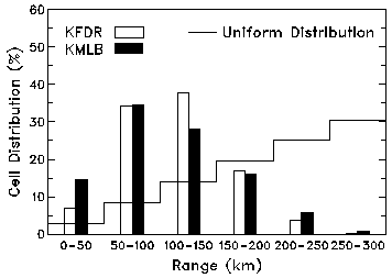
Figure 1. Distribution of radar-detectable cells at 50-km intervals for the KFDR and KMLB data sets. The stepped line is the distribution that would arise if cells were uniformly distributed within 300 km range of a radar.

We evaluated the utility of VCP 22 by comparing its algorithm output with that of VCP 11. The values of algorithm parameters used for the comparisons came from "fort.nn" files that were written to disk when the algorithms were run on the radar data sets. The severe weather algorithms and parameters that were selected for comparison are:

WSR-88D Storm Cell Identification and Tracking (SCIT) Algorithm -- maximum reflectivity, height of maximum reflectivity, height of 30-dBZ reflectivity contour

WSR-88D Vertically Integrated Liquid (VIL) Algorithm (cell-based) -- VIL

WSR-88D Hail Detection Algorithm (HDA) -- probability of hail, probability of severe hail, maximum expected hail size

WSR-88D Mesocyclone Algorithm (MESO) -- mesocyclone depth, maximum rotational velocity, maximum azimuthal shear, integrated rotational strength index

NSSL Mesocyclone Detection Algorithm (MDA) -- mesocyclone depth, maximum rotational velocity, maximum azimuthal shear, mesocyclone strength rank, mesocyclone strength index

NSSL Tornado Detection Algorithm (TDA) -- signature depth, maximum gate-to-gate velocity difference, maximum gate-to-gate shear

NSSL Neural Network (NN) Probabilities -- probability of tornado, probability of severe winds

NSSL's Damaging Downburst Prediction and Detection Algorithm (DDPDA) was not evaluated for two reasons. First, the same features were detected using VCP 11 and VCP 22 because detections are based on divergence at the common lowest elevation angle. Second, no predictions (which are based on mid-altitude features) were produced by the algorithm for either data set.

The WSR-88D algorithm for estimating rainfall (Fulton et al. 1998) was not used to assess VCP 22 because the algorithm is based on measurements at the four lowest elevation angles, which are the same for VCP 11 and 22. An attempt was made, however, to run the algorithm on VCP 22 data. We had to change the VCP number in the algorithm before it would run using VCP 22 data. The algorithm did not produce any one-hour or three-hour rainfall accumulations for VCP 22 owing to the 32/3-min volume scans. However, the algorithm did produce storm total precipitation amounts, but the VCP 22 amounts were 73% (= 32/3 min / 5 min) of those produced by VCP 11.

3. Storm Cell Identification and Tracking (SCIT) Algorithm

The SCIT algorithm identifies the existence and characteristics of individual storm cells (e.g., Johnson et al. 1998). The algorithm also tracks and forecasts the three-dimensional centroid positions of the cells. In this study, we could not devise an objective way to evaluate the effect of VCP 22 on cell identification and tracking. However, inspection of the displayed tracks indicated that the vast majority of identified cells and their tracks were identical.

A comparison of maximum reflectivity, height of the maximum reflectivity and top of the 30-dBZ reflectivity contour using VCP 11 and VCP 22 is found in Figs. 2-4. Data for KMLB are plotted in the top half of each figure and data for KFDR are plotted in the bottom half. The left panels show scatter plots of values for the two VCPs. The differences between the VCP 11 and VCP 22 values are plotted as a function of range in the right panels. One may note that the differences between the parameter values at greater ranges are zero because all of the pertinent data are at common elevation angles below 5.0o (see Table 1).

Listed in the upper left corner of each panel are the number of VCP 11 data points, the number of VCP 22 data points and the number of VCP 11 and 22 data point pairs that occurred at the same range and azimuth for a given volume scan. Listed in the bottom right corner of the left panels are the number of paired data points where the VCP 11 value is greater than, equal to or less than the VCP 22 value. Listed in the bottom right corner of each right panel are the same numbers as in the left panels, but they are expressed in terms of differences between the VCP 11 and 22 values.

Plots of maximum reflectivity values within each storm are shown in Fig. 2. With one or two exceptions, the VCP 22 values (Max Z22) are less than or equal to VCP 11 values (Max Z11). This relationship is expected since some of the VCP 11 maximum reflectivity values will occur at elevation angles that are missing in VCP 22.

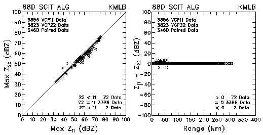
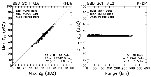
Figure 2. Plots of maximum reflectivity values and reflectivity differences between VCP 11 and VCP 22 for data collected by KMLB and KFDR.

Plots of the height of maximum reflectivity values are shown in Fig. 3. Of the few pairs that do not have the same values, most of the VCP 22 values underestimate those associated with VCP 11. This relationship again is to be expected owing to the missing elevation angles with VCP 22.

Owing to the missing VCP 22 elevation angles, there are four distinct elevation angle differences that can arise between VCP 11 elevation angles and the closest VCP 22 elevation angle: 0.95o, 1.3o, 2.0o, 2.5/2.7/2.8o (consult Table 1). One may note in Fig. 3 that some of the plotted values appear to be concentrated into bands radiating outward from the origin. The bands in this figure are associated with elevation angle differences of 0.95o.

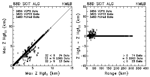
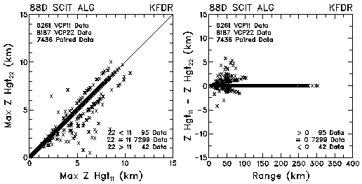
Figure 3. Plots of heights of maximum reflectivities and height differences between VCP 11 and VCP 22 for data collected by KMLB and KFDR. The cause of the radial bands is discussed in the text.

Plots of the heights of the tallest 30-dBZ features in the storms are shown in Fig. 4. For nearly all of the pairs where the heights are not equal, the VCP 22 tops are lower than the VCP 11 tops. The missing elevation angles with VCP 22 can account for this situation. It is not clear why VCP 22 tops are higher in about 0.5% of the cases.

The dense radial bands in Fig. 4 are more pronounced than in Fig. 3. The dense band in the KMLB data is due to a combination of elevation angle differences of 0.95o and 1.3o. The two dense bands in the KFDR data is due to a combination of 0.95o and 1.3o and to 2.5/2.7/2.8o. The radial bands of concentrated data points occur only with height parameters. Several parameters presented in later figures are for the depth of features. Since there are many combinations of elevation differences that can specify depth, none of the depth plots have unique radial bands.

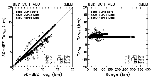
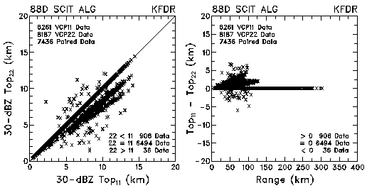
Figure 4. Plots of the heights of 30-dBZ tops of storm cells and height differences between VCP 11 and VCP 22 for data collected by KMLB and KFDR. The cause of the radial bands is discussed in the text.

4. Vertically Integrated Liquid (VIL) Algorithm

Vertically integrated liquid (VIL) is a measure of the liquid water in a vertical column in the storm. It is computed as a function of the vertical profile of reflectivity (Greene and Clark 1972). Instead of VIL being computed in vertical columns, as originally proposed, it is computed in this algorithm from the maximum reflectivity at each level within an identified storm cell. This "cell-based" approach takes into account tilting reflectivity cores (e.g., Johnson et al. 1998).

Plots of cell-based VIL are shown in Fig. 5. For those VIL values that are not equal for VCP 11 and 22, most of the ones associated with VCP 22 are greater (by 10-20 kg m-2) than those associated with VCP 11. Initially this may seem to be a bit strange, since VCP 22 has a few deleted elevation angles. However, as part of the vertical integration process, the maximum reflectivity at each elevation angle is assigned to a depth extending from halfway to the adjacent lower elevation angle to halfway to the adjacent higher elevation angle. If the maximum reflectivity in the storm occurs at one of the VCP 22 elevation angles above 5o, that value will be assigned to a greater depth than for the same VCP 11 elevation angle.

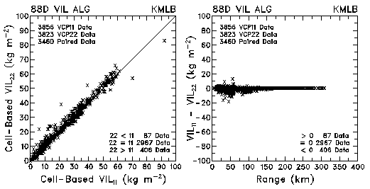
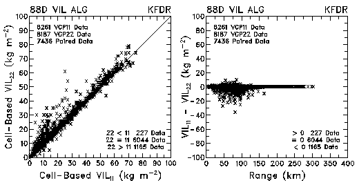
Figure 5. Plots of VIL and VIL differences between VCP 11 and VCP 22 for data collected by KMLB and KFDR.

5. WSR-88D Hail Detection Algorithm (HDA)

Characteristics of the WSR-88D Hail Detection Algorithm (HDA) are discussed by Witt et al. (1998). We investigated three parameters produced by HDA: probability of hail, probability of severe hail and maximum expected hail size. Comparisons of the parameters using VCP 11 and VCP 22 are found in Figs. 6-8.

Probability of hail (POH) of any size is computed as a function of the height of the 45-dBZ echo above the environmental freezing level. Plots of the probability are shown in Fig. 6. In the left half of the figure, nearly all of the comparison data points fall on the diagonal 1:1 line. As listed in the bottom right corner of the panels, about half of the points along the 1:1 line are at the origin where POH22 = POH11 = 0%. In the right half of the figure, the few points that do not have the same probability are equally scattered on both sides of the zero line for KMLB. However, there are more cases where the VCP 11 values are greater than VCP 22 values for KFDR. Typical differences in probability between the two VCPs is about 10%.

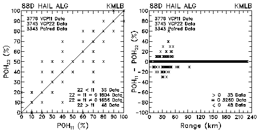
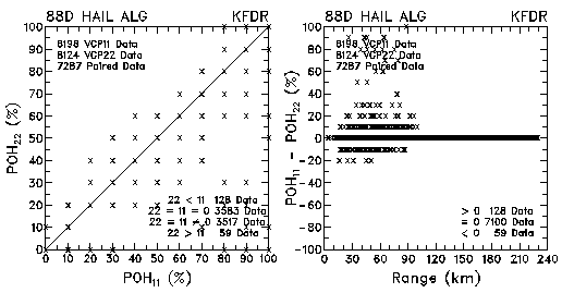
Figure 6. Plots of probability of hail (POH) and probability differences between VCP 11 and VCP 22 for data collected by KMLB and KFDR.

The probability of severe hail (POSH; diameter 1.9 cm or 0.75 in) is a function of the vertical integration of an empirical function of maximum reflectivity values 40 dBZ (Witt et al. 1998). Plots of POSH are shown in Fig. 7. The distributions are similar to those for POH, with the typical differences between the two VCPs being about 10%.

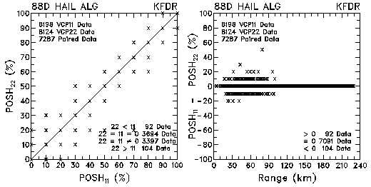
Figure 7. Plots of probability of severe hail (POSH) and probability differences between VCP 11 and VCP 22 for data collected by KMLB and KFDR.

The prediction of maximum expected hail size, like POSH, is a function of the vertical integration of an empirical function of maximum reflectivity values 40 dBZ. Plots of maximum expected hail size are found in Fig. 8. There is relatively little difference in expected hail size between the two VCPs. In fact, the typical extreme differences are only 0.6 cm (0.25 in).

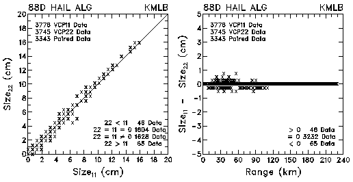
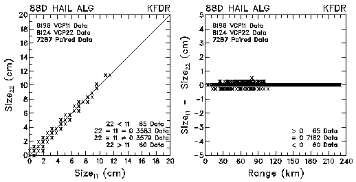
Figure 8. Plots of maximum expected hail size and size differences between VCP 11 and VCP 22 for data collected by KMLB and KFDR.

6. WSR-88D Mesocyclone Algorithm (MESO)

The WSR-88D Mesocyclone Algorithm identifies cyclonic circulations that exceed specified shear and height criteria. In this report, we investigate four parameters produced by the algorithm: mesocyclone depth, maximum rotational velocity, maximum azimuthal shear across the mesocyclone and the integrated rotational strength index. Comparisons of the parameters using VCP 11 and VCP 22 are plotted in Figs. 9-12.

Mesocyclone depth is computed over a depth of at least 3 km (10 kft) where the shear exceeds a specified threshold value; a vertical gap where the shear drops below the threshold value is permitted. Plots of mesocyclone depth are shown in Fig. 9. Of the depths that are not the same for the two VCPs, those computed from VCP 11 are almost always greater. One would expect to find this type of relationship because the top of the mesocyclone feature at times will fall at the height of a missing elevation angle in VCP 22.

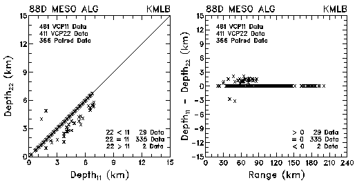
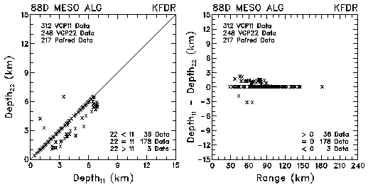
Figure 9.Plots of mesocyclone depth and depth differences between VCP 11 and VCP 22 for data collected by KMLB and KFDR. The plots are based on the WSR-88D Mesocyclone Algorithm.

The rotational velocity at a given elevation angle is computed as one-half the difference between the maximum Doppler velocity value and the minimum Doppler velocity value across the mesocyclone signature. The maximum rotational velocity for the three-dimensional feature is the maximum of the rotational velocities at the various elevation angles.

Plots of the maximum rotational velocity are shown in Fig. 10. Differences in maximum rotation velocity between the two VCPs is minimal. Where differences occur, the VCP 11 values are almost always greater than the VCP 22 values. This is to be expected, again owing to the missing elevation angles with VCP 22.

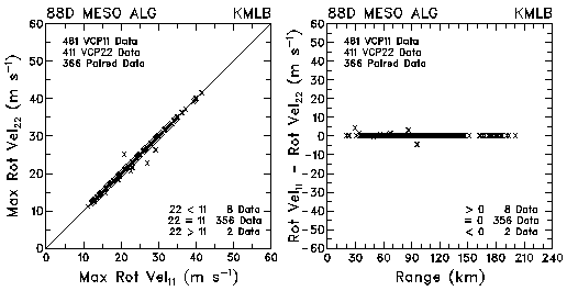
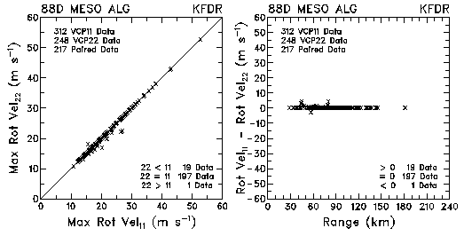
Figure 10. Plots of maximum rotational velocity and velocity differences between VCP 11 and VCP 22 for data collected by KMLB and KFDR. The plots are based on the WSR-88D Mesocyclone Algorithm.

At a given elevation angle, shear is computed as the difference between the extreme Doppler velocity values across the mesocyclone signature divided by the distance between the extreme values. Plotted in Fig. 11 are the maximum shear values throughout the mesocyclone depth. Only a few per cent of the shear values are not the same for the two VCPs. Where there are differences, VCP 11 values are larger in almost all cases.

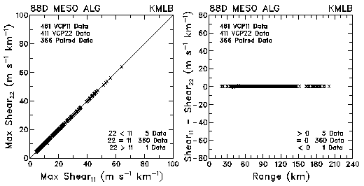
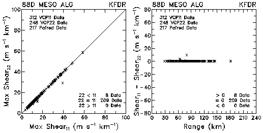
Figure 11. Plots of maximum shear and shear differences between VCP 11 and VCP 22 for data collected by KMLB and KFDR. The plots are based on the WSR-88D Mesocyclone Algorithm.

A rotational shear index is computed from a nomogram based on the rotational velocity and diameter of the mesocyclone signature at a given elevation angle (Lee and White 1998). The integrated rotational shear (IRS) index is the sum of the individual rotational shear index values with height. Plotted in Fig. 12 are IRS index values. Where there are differences, larger IRS index values are associated with VCP 11. Again, this situation is to be expected owing to the missing elevation angles with VCP 22.

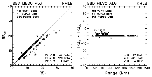
Figure 12. Plots of integrated rotational strength (IRS) index and IRS index differences between VCP 11 and VCP 22 for data collected by KMLB and KFDR. The plots are based on the WSR-88D Mesocyclone Algorithm.

7. NSSL Mesocyclone Detection Algorithm (MDA)

The NSSL Mesocyclone Detection Algorithm (MDA) is a not-yet-operational enhancement of the WSR-88D Mesocyclone Algorithm (Stumpf et al. 1998). We investigated five parameters produced by the NSSL algorithm: mesocyclone depth, maximum rotational velocity, maximum azimuthal shear across the mesocyclone, three-dimensional mesocyclone strength rank and mesocyclone strength index (MSI). The data presented in Figs. 13-17 are from those mesocyclones that had a strength rank of at least 5.

Mesocyclone depth is computed from the unbroken sequence of elevation angles at which a two-dimensional mesocyclone signature is identified. Since weaker mesocyclone signatures are available from the NSSL algorithm than from the WSR-88D algorithm, vertical gaps do not need to be considered in establishing vertical continuity of a feature.

Plotted in Fig. 13 are mesocyclone vertical depths from the NSSL algorithm. There are greater differences between the two VCPs than with the WSR-88D depths in Fig. 9. Also, fewer mesocyclones are identified when the NSSL strength rank of 5 is used.

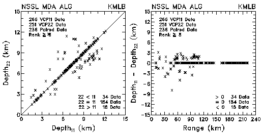
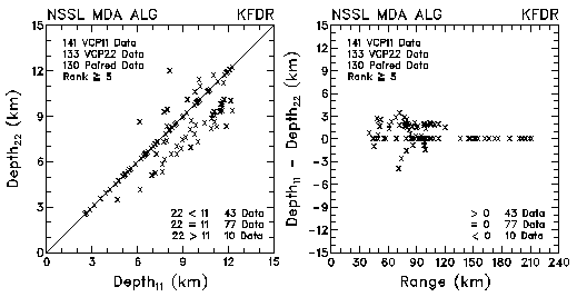
Figure 13. Plots of mesocyclone depth and depth differences between VCP 11 and VCP 22 for data collected by KMLB and KFDR. The plots are based on the NSSL Mesocyclone Detection Algorithm.

The NSSL Mesocyclone Detection Algorithm is more realistic than its WSR-88D counterpart in finding the peak Doppler velocity values of the mesocyclone signature. The NSSL algorithm allows for small-scale increases and decreases in the velocity field as the algorithm starts at the velocity minimum and searches from the velocity maximum. This approach produces more representative values of maximum rotational velocity, mesocyclone core diameter and maximum shear.

Plotted in Fig. 14 are the maximum rotational velocities from the NSSL algorithm. The differences in values between the two VCPs are not very great and are comparable to those found with the WSR-88D algorithm (Fig. 10). For most of the differences, VCP 11 values are greater than those for VCP 22, which is to be expected.

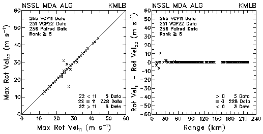
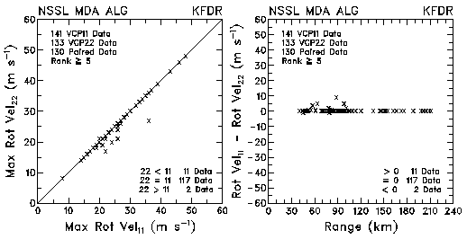
Figure 14. Plots of maximum rotational velocity and velocity differences between VCP 11 and VCP 22 for data collected by KMLB and KFDR. The plots are based on the NSSL Mesocyclone Detection Algorithm.

Plotted in Fig. 15 are the maximum shear values from the NSSL Mesocyclone Detection Algorithm. About 10% of the paired shear values are different for the two VCPs, which is much greater than for the WSR-88D algorithm (Fig. 11). In virtually all cases, the VCP 11 shears are greater than the those for VCP 22. This relationship is to be expected owing to the missing elevation angles of VCP 22.

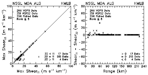
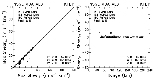
Figure 15. Plots of maximum shear and differences in shear values between VCP 11 and VCP 22 for data collected by KMLB and KFDR. The plots are based on the NSSL Mesocyclone Detection Algorithm.

The mesocyclone signature at each elevation angle is assigned a two-dimensional (2D) strength rank based on threshold values of the Doppler velocity difference across the signature or of the shear across the signature, depending on which one is rated higher (for details see Stumpf el al. 1998). The threshold values decrease with increasing range to reflect sampling problems associated with the broadening of the radar beam with range. The overall strength rank for the three-dimensional (3D) mesocyclone is determined "by finding the strongest continuous vertical core of 2D features whose 2D strength ranks are greater than or equal to a given strength rank. This core must be at least 3 km [9.8 kft] in half-beamwidth depth, and the base of the core must be below 5 km [16.4 kft]" (Stumpf et al. 1998).

Plotted in Fig. 16 are the 3D strength ranks. Only about 3% of the values are not the same for the two VCPs and, for most of these, the VCP 11 value is greater. If some of the larger 2D strength ranks were at the missing elevation angles of VCP 22, one would expect the VCP 22 3D values to be less than or equal to those for VCP 11.

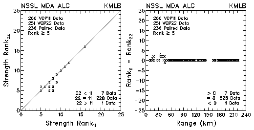
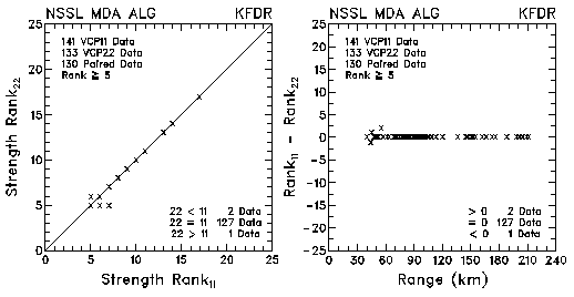
Figure 16. Plots of 3D strength rank and differences in strength rank between VCP 11 and VCP 22 for data collected by KMLB and KFDR. The plots are based on the NSSL Mesocyclone Detection Algorithm.

The ultimate classification of a mesocyclone with the NSSL algorithm is the mesocyclone strength index (MSI). The MSI is computed by vertically integrating the strength ranks (multiplied by 1000) of each 2D feature, which is weighted by the air density at the height of the feature. This means that 2D features at lower heights are given more weight. In order to normalize the MSI values for a variety of mesocyclone depths, the MSI is divided by the total 3D depth of the feature.

Plotted in Fig. 17 are the MSI values. About 25-30% of the paired values are different for the two VCPs. In most cases, the VCP 11 values are greater.

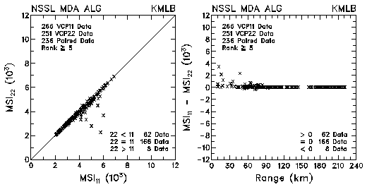
Figure 17. Plots of mesocyclone strength index (MSI) and differences in index values between VCP 11 and VCP 22 for data collected by KMLB and KFDR. The plots are based on the NSSL Mesocyclone Detection Algorithm.

8. NSSL Tornado Detection Algorithm (TDA)

The NSSL Tornado Detection Algorithm (TDA) is designed to identify the locally intense vortices measured by the WSR-88D that are associated with tornadoes (e.g., Mitchell et al. 1998). Brown et al. (1978) point out that when the radar beam is larger than the tornado, a degraded version of the tornado is evident in the Doppler velocity measurements. They called the degraded signature a Tornadic Vortex Signature (TVS). This algorithm divides the TVS into two subcategories. "A 3D detection is classified as a TVS if it meets minimum strength and depth criteria and if the base extends to the 0.5o elevation angle or a prescribed altitude ARL (currently 600 m). Otherwise, a 3D detection that meets the TVS criteria except for the base elevation or altitude criterion" is called an elevated TVS (ETVS) (Mitchell et al.).

In this report, we investigate three algorithm parameters: TVS depth, maximum gate-to-gate azimuthal velocity difference and maximum azimuthal shear. Both TVS and ETVS occurrence are included in the results. Comparisons of the parameters using VCP 11 and VCP 22 are found in Figs. 18-20.

The vertical depth of a 3D (E)TVS is defined by at least two adjacent elevation angles that have vertically-correlated 2D features; no more than one gap, where data are missing or the prescribed 2D vortex criteria are not met, is permitted in the vertical. Plotted in Fig. 18 are (E)TVS depths based on VCP 11 and VCP 22. About 20-30% of the data points are different for the two VCPs. In a vast majority of these cases, VCP 11 depths are greater than VCP 22 depths. These differences would occur if a portion of the 3D (E)TVS occurs at an elevation angle that is missing in VCP 22. In both Florida and Oklahoma, (E)TVSs are identified up to 150 km (81 n mi) from the radar.

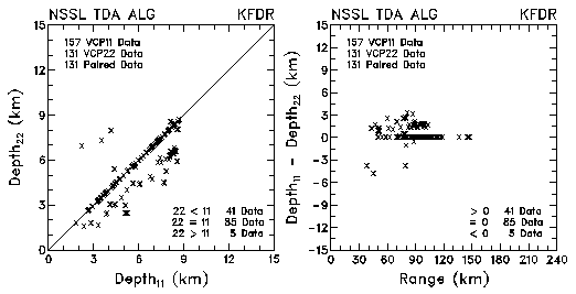
Figure 18. Plots of (E)TVS depth and differences in depth values between VCP 11 and VCP 22 for data collected by KMLB and KFDR. The plots are based on the NSSL Tornado Detection Algorithm.

The conventional feature that indicates the presence of a (E)TVS in the Doppler velocity display at a given elevation is a marked 2D Doppler velocity difference at range gate locations that are adjacent in azimuth. The maximum gate-to-gate azimuthal Doppler velocity differences in the 3D feature for VCP 11 and VCP 22 are plotted in Fig. 19. With few exceptions, the velocity differences are the same for both VCPs. Where there are VCP differences, VCP 11 values are larger in nearly every instance.

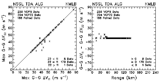
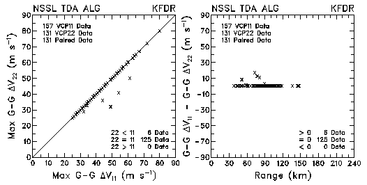
Figure 19. Plots of maximum gate-to-gate azimuthal Doppler velocity differences and differences in the velocity difference values between VCP 11 and VCP 22 for data collected by KMLB and KFDR. The plots are based on the NSSL Tornado Detection Algorithm.

The azimuthal shear associated with a (E)TVS is defined as the Doppler velocity difference at azimuthally adjacent range gates (that is, gate-to-gate difference) divided by the azimuthal distance between the two gates. Plotted in Fig. 20 are the maximum azimuthal shear values within the 3D (E)TVS. The vast majority of values are the same for the two VCPs. When there are differences, VCP 11 values are nearly always larger.

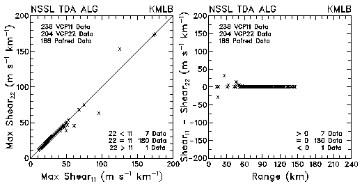
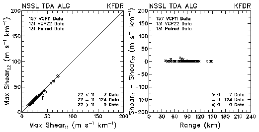
Figure 20. Plots of maximum azimuthal shear and differences in the shear values between VCP 11 and VCP 22 for data collected by KMLB and KFDR. The plots are based on the NSSL Tornado Detection Algorithm.

9. NSSL Neural Network (NN) Probabilities

Given a large data set of nonlinearly-related parameters, a neural network can be trained to reveal otherwise hidden relationships. Marzban and Stumpf (1996) used a neural network to derive relationships between the characteristics of mesocyclones detected by Doppler radar and the probability of tornadoes (POT).

Plotted in Fig. 21 are comparisons of the probability of tornado occurrence using VCP 11 and VCP 22 data from the KMLB and KFDR radars. Much of the scatter in the diagram can be attributed to an inherent statistical uncertainly of 5-10% in the individual probability values. Both VCPs had 0% probability of tornadoes for 56% of the paired KMLB data points and 74% of the KFDR data points. Of the remaining data points, the two VCPs produced equal probabilities for about half of them. Of the data points where the probabilities were not equal, VCP 11 had higher probabilities in about 70% of the cases. Where there were differences, most of the VCP 22 results differed from VCP 11 results by roughly 10-15% probability.

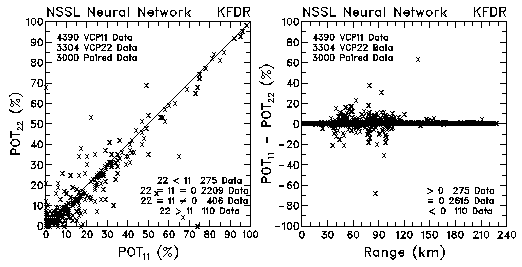
Figure 21. Plots of probability of tornado occurrence (POT) and probability differences between VCP 11 and VCP 22 for data collected by KMLB and KFDR.

Marzban and Stumpf (1998) used a neural network to derive relationships between the characteristics of mesocyclones detected by Doppler radar and the probability of severe winds (POSW). Plotted in Fig. 22 are comparisons of the probability of severe wind occurrence using VCP 11 and VCP 22 data from the KMLB and KFDR radars. Both VCPs had 0% probability of severe wind for 47% of the paired KMLB data points and 62% of the KFDR data points. Of the remaining data points, the two VCPs produced equal probabilities for about half of them. Of the data points where the probabilities were not equal, VCP 11 had higher probabilities in about 70% of the cases. Where there were differences, most of the VCP 22 results differed from VCP 11 results by roughly 20% probability for KMLB and by roughly 15% probability for KFDR.

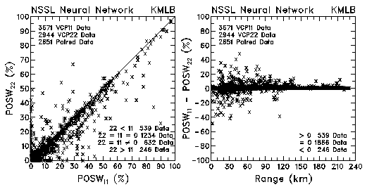
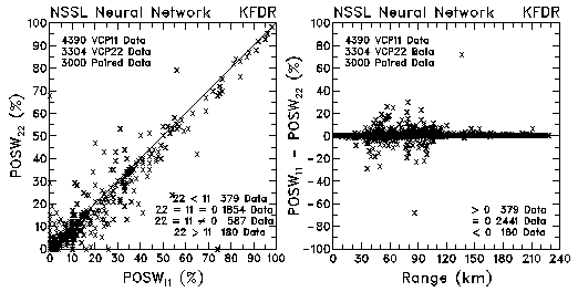
Figure 22. Plots of probability of severe winds (POSW) and probability differences between VCP 11 and VCP 22 for data collected by KMLB and KFDR.

10. Velocity Azimuth Display (VAD) Algorithm

When a Doppler radar makes a 360o scan at a constant elevation angle and there is sufficient radar return at a given slant range over portions of the scan, it is possible to retrieve the mean wind direction and speed around the slant range circle centered on the radar location (e.g., Lhermitte and Atlas 1961). A vertical profile of wind direction and speed can be obtained from the full set of elevation angles specified by a given VCP. For the WSR-88D VAD Algorithm, a vertical profile is constructed at a range of 30 km (16.2 n mi). The heights at which winds are desired are specified. Then the elevation angle at each height that is closest to 30-km range is used for the wind computations. For this study, the VCP number and elevation angles had to be hardwired in the code in order for the algorithm to run on VCP 22 data.

Plotted in Fig. 23 are the VAD wind directions for VCP 11 and 22. The plots in the left half of the figure indicate some scatter about the 1:1 line. The plots in the right half of the figure reveal the reason for the scatter. VAD wind directions computed from the elevation angles that are common to both VCPs are exactly the same. However, at heights corresponding to the missing VCP 22 elevation angles, the wind directions are different. The differences arise from the fact that, at a given height, the VCP 22 elevation angle closest to the range of 30 km is not the same as the closest VCP 11 elevation angle. Most VCP 22 wind directions are within 10o of the VCP 11 directions.

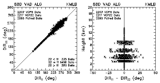
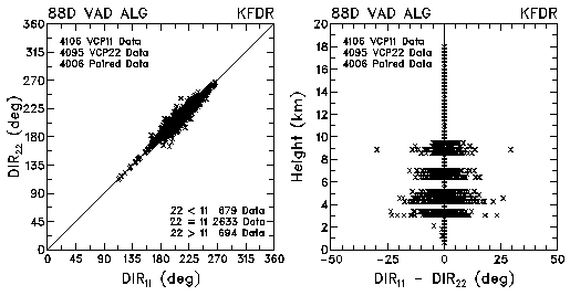
Figure 23. Plots of VAD wind direction and direction differences between VCP 11 and VCP 22 for data collected by KMLB and KFDR. Heights are relative to sea level.

Plotted in Fig. 24 are VAD-derived wind speeds for VCP 11 and 22. As with wind direction in Fig. 23, the wind speed differences occur at the heights of missing elevation angles in VCP 22. On the whole, most VCP 22 wind speeds are within 3-4 m s-1 (6-8 kt) of the VCP 11 speeds.

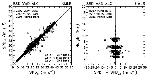
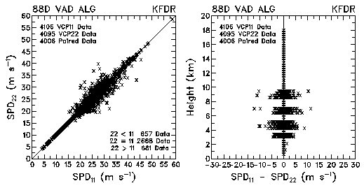
Figure 24. Plots of VAD wind speed and speed differences between VCP 11 and VCP 22 for data collected by KMLB and KFDR. Heights are relative to sea level.

11. Concluding Comments

The most obvious way, but not only way, to increase the temporal resolution of WSR-88D data is to decrease the vertical resolution of a VCP. That is the approach used in this study. We modified VCP 11 by deleting five elevation angles, so the remaining elevation angles would closely resemble VCP 21. The modified version of VCP 11 (which we call VCP 22) takes 32/3 min to complete a volume scan compared to 5 min for VCP 11. Using VCP 22 as a proxy for VCP 21, we have compared algorithm output using VCP 11 and VCP 21/22. Considering that some of the elevation angles present in VCP 11 are missing from VCP 21/22, we appropriately find that the algorithm output that forecasters depend on for issuing warnings is noticeably compromised.

The data presented in Figs. 2-20 indicate that algorithm output from VCP 11 and VCP 22 are identical at far ranges where elevation angles are below 5o; that is, where VCP 11 and VCP 21/22 have common elevation angles (see Table 1). However, differences in values of algorithm parameters can occur when the heights of specific parameters are above 5o elevation. From the data presented in the figures, one is not able to determine how many of the paired data points above 5o elevation are the same and how many are different.

Figure 25 was prepared to investigate the percentage of paired data points above 5o that are different. The following six algorithm parameters are not included in Fig. 25 because the height of the maximum value, from which an elevation angle could be computed, was not available: probability of hail (POH, Fig. 6), maximum rotational velocity (Fig. 10) and maximum shear (Fig. 11) from the WSR-88D Mesocyclone Algorithm, strength rank (Fig. 16) from the NSSL Mesocyclone Detection Algorithm, and probability of tornado occurrence (POT, Fig. 21) and probability of severe winds (POSW, Fig. 22) from the neural network. The five parameters with asterisks are those derived through vertical integration of various quantities and therefore do not have a height associated with them. To compute representative elevation angles for the asterisked parameters, the 30-dBZ top height was used as the top of the VIL and hail parameters and the respective heights of mesocyclone tops were used for the WSR-88D and NSSL mesocyclone parameters.

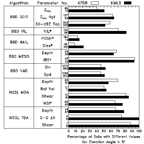
Figure. 25. Percentage of algorithm parameter values that were different using VCP 11 and VCP 21/22 when the elevation angle of the parameter was greater than 5o; missing elevation angles above 5o for VCP 21/22 produce the different values. The numbers in the third column are the number of paired data points that were different for each radar. Asterisks indicate those parameters that arise from vertical integration; the 5o threshold applies to the top of the integration column.

The bars in Fig. 25 indicate that, on the average, over half of the paired data points above 5o elevation derived from VCP 21/22 are different from those derived from VCP 11. The number of paired data points that were different for each parameter are listed in the third column. These differences can seriously mislead forecasters into not issuing warnings that should have been issued or issuing warnings that should not have issued. Even though it is faster than VCP 11, the degradation in vertical resolution associated with VCP 21/22 typically underestimates the strength of mesocyclone and tornadic vortex signatures. Also, underestimating mesocyclone or TVS depth could mean that the vortex misses being identified as a mesocyclone or TVS. VIL, the only parameter that is systematically overestimated, is a popular parameter for evaluating storm severity. Forecasters could issue needless warnings when VCP 21 data indicate a VIL value that is 10-20 kg m-2 too large. Based on the results of this comparative study, we recommend that VCP 22 not be implemented. (In fact, we see no reason why VCP 21 should be used in severe weather situations, since it has less temporal and vertical resolution than VCP 11.)

In lieu of implementing "VCP 22", we recommend that the OSF await the results of MOU Task 8.2, which will be completed in January 1999. For Task 8.2, we are developing a suite of VCPs designed to improve the temporal and spatial resolution of a spectrum of convective storms. However, there are some practical drawbacks to implementing faster VCPs at the present time. During the course of this study, we have found that the WSR-88D algorithm for estimating rainfall does not function properly when the number of volume scans we were not able to get any one-hour or three-hour rainfall totals and the storm totals were 73% (equal to 32/3 min / 5 min) of the VCP 11 amounts. Therefore, software changes need to be made to the rainfall algorithm before any faster VCPs can be added to the WSR-88D system. When faster algorithms are developed, they need to be tested at forecast offices to see whether they cause any real-time interpretation problems.

This report documents the importance of comparing different VCPs and different versions of the same algorithms using a common set of WSR-88D data. We were fortunate in this case that a reasonable facsimile of VCP 21 could be constructed from VCP 11. This will not be the case when we want to compare new and old VCPs in the future. We recommend that several special data sets be collected that have unusually dense data in the vertical. Proxy VCPs then could be constructed by interpolating the denser data to the desired elevation angles. In this way, some standardized procedures could be established for evaluating new VCPs.

References

Brown, R. A., L. R. Lemon and D. W. Burgess, 1978: Tornado detection by pulsed Doppler radar. Mon. Wea. Rev., 106, 29-38.

Fulton, R. A., J. P. Breidenbach, D.-J. Seo, D. A. Miller and T. O'Bannon, 1998: The WSR-88D rainfall algorithm. Wea. Forecasting, 13, 377-395.

Greene, D. R., and R. A. Clark, 1972: Vertically integrated liquid: A new analysis tool. Mon. Wea. Rev., 100, 548-552.

Johnson, J. T., P. L. MacKeen, A. Witt, E. D. Mitchell, G. J. Stumpf, M. D. Eilts and K. W. Thomas, 1998: The storm cell identification and tracking algorithm: An enhanced WSR-88D algorithm. Wea. Forecasting, 13, 263-276.

Lee, R. R., and A. White, 1998: Improvement of the WSR-88D mesocyclone algorithm. Wea. Forecasting, 13, 341-351.

Lhermitte, R. M., and D. Atlas, 1961: Precipitation motion by pulse Doppler radar. Proc. Ninth Wea. Radar Conf., Amer. Meteor. Soc., 218-223.

Marzban, C., and G. J. Stumpf, 1996: A neural network for tornado prediction based on Doppler radar-derived attributes. J. Appl. Meteor., 35, 617-626.

_____, and _____, 1998: A neural network for damaging wind prediction. Wea. Forecasting, 13, 151-163.

Mitchell, E. D., S. V. Vasiloff, G. J. Stumpf, A. Witt, M. D. Eilts, J. T. Johnson and K. W. Thomas, 1998: The National Severe Storms Laboratory tornado detection algorithm. Wea. Forecasting, 13, 352-366.

Stumpf, G. J., A. Witt, E. D. Mitchell, P. L. Spencer, J. T. Johnson, M. D. Eilts, K. W. Thomas and D. W. Burgess, 1998: The National Severe Storms Laboratory mesocyclone detection algorithm for the WSR-88D. Wea. Forecasting, 13, 304-326.

Witt, A., M. D. Eilts, G. J. Stumpf, J. T. Johnson, E. D. Mitchell and K. W. Thomas, 1998: An enhanced hail detection algorithm for the WSR-88D. Wea. Forecasting, 13, 286-303.