Lightning Data - General Discussion
Source:
The lightning data used on this page comes from
the National Lightning Detection Network (NLDN), operated by Global Atmospherics,
Inc [ http://www.glatmos.com
]. The NLDN detects cloud to ground lightning strikes across the
US with a network of over 100 sensors. More technical information on how
this is done can be found in the following reference [1]:
[K.L.Cummins, E.A.Bardo, W.L.Hiscox, R.B.Pyle, A.E.Pifer NLDN '95: A
Combined TOA/MDF Technology Upgrade of the U.S. National Lightning Detection
Network from the Proceedings of the 12th Conference of Interactive Information
and Processing Systems (IIPS) For Meteorology, Oceanography, and Hydrology]
The NLDN has been in operation since 1989.
Initially, strike locations were estimated to be only accurate to a rather
coarse 10 km. Upgrades occured in the early 90's and by 1995 there
was a significant increase in both detection efficiency and location accuracy.
The detection efficiency (the percentage of the actual strikes that are
detected by the network) is reported to be 80%-90%. The reported
locations of strikes are accurate on average to about 0.5 km. This
resolution raised, for the first time, the possibility of correlating lightning
with terrain features on a fairly fine scale; for instance, the scale of
a mountain ridgeline, a canyon edge, an isolated desert mountain peak or
even an isolated tall tower. The decision was made to not use the less
accurate NLDN data from before 1995 in the analysis here. Currently
the data used in this work runs from Jan 1, 1995 to Dec 31, 1999.
The times of day reported in the original NLDN data are UCT, but for all
of the work done here the times were converted to (MST) time.
A small sample fragment of NLDN data is shown
below:
09/30/95 23:56:57 34.834 -113.248 0.0 -20.4 kA 2
09/30/95 23:56:58 32.063 -111.071 0.0 -10.2 kA 1
09/30/95 23:57:58 34.329 -110.970 0.0 38.0 kA 1
09/30/95 23:59:59 34.879 -113.354 0.0 -35.9 kA 12
The first four data fields present are Date, Time, Latitude, and Longitude.
The last two give the Peak Current (including polarity) and the Multiplicity
of strokes per flash. To correlate lightning with terrain, an additional
data field that would be of interest would be the elevation at which the
strike occured. Computer code was written to use a strike's latitude
and longitude to lookup and assign an elevation to each strike. The
elevations came from the U.S. Geological Survey datasets called Digital
Elevation Models (DEM's) [see: Elevation
Data - General Discussion ]. The NLDN data reports lightning
strike latitude and longitude to the nearest 0.001 degree. This corresponds
to 3.6 arcsec, which is close to the 3 arcsec resolution of the elevation
data found in the USGS DEM's. A resolution of 3.6 or 3.0 arcsec would pinpoint
a location to within about 100 m, but the error bars on the lightning location
are actually larger. The average accuracy of the strike location is more
like 500 m.
The image below illustrates the situation. The fine
grid represents 3 arcsec latitude and longitude bins. A strike is reported
at the red 'x', but there is a 50 % chance that the actual location is
somewhere within the small red ellipse and a 90% chance it is within the
larger ellipse (see Ref. [1] above).
Region and Period of Study:
This study covers the 72 quadrangles from
latitude 31 N to 43 N and longitude 114 W to 108 W. This includes
virtually all of Arizona (except a slender strip bordering Calif.), all
of Utah, New Mexico and Colorado and pieces of Idaho, Wyoming and Nebraska.
The 72 quad region is quartered into sections of 6 quads north to south
by 3 quads east to west. This division correpsonds approximately
to the four states of Arizona, Utah, Colorado and New Mexico. Those
four regions will be referred to by those titles, but it should
be kept in mind that the 'Arizona' region contains a slice of far western
New Mexico, the 'Colorado' region contains parts of Wyoming and Nebraska
and so on.
The study is limited to the summer monsoon months
of July and August. To see how this season fits into the larger picture,
the following graphic shows a plot of the monthly total lightning for each
of the four state regions for the whole year. The number of strikes
is a total for that month for the five year period 1995-1999. 1 =
Jan., 2 = Feb. and so on.
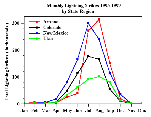
The bulk of the lightning occurs in the summer monsoon
period of July and August, when 67% of the annual lightning occurs.
Again, this is the period of interest in the study. Of the
rest of the year, by far the next biggest contribution is from September
or June. However, in September storm systems from the Pacific often
begin to play a role and in June the high plains are more active so the
signal begins to contain more than just the summer monsoon pattern.
In July and August, Arizona and New Mexico dominate
the lightning count. The numbers are not adjusted to reflect density,
which provides a small bias, but this only amounts to about 5% of the enhancement
of the southern tier of states. (All four regions cover the same
size rectangle in terms of latitude and longitude, but the area on the
ground is less for the more northern regions due to the curvature of the
earth.) New Mexico and Colorado both cover a large area of
high plains, so they dominate in May and June. It is interesting
to note that Arizona and New Mexico are both strong in July and August,
but are roughly mirror image in terms of a slight August peak for Arizona
and a slight July peak for New Mexico. Lightning in Colorado doesn't
strongly favor July or August and Utah has fairly constant counts for July,
August and September.
Display Options:
With the lightning data chosen, the question arises
as to how to display the data. The lightning strike locations are
given to the nearest 0.001 degree latitude and longitude. This
is close to 100 m distance, however the typical error in these locations
are more like 500 m. The following image shows the southwest corner
of the Santa Catalina mountains NE of Tucson:
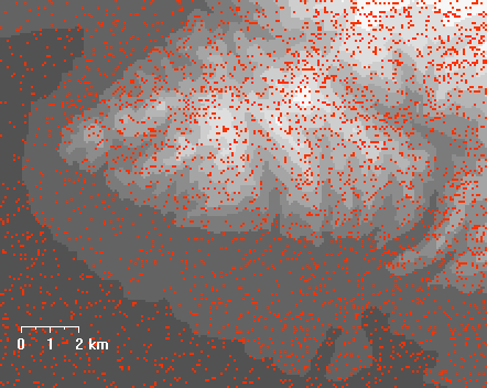 Each red dot is a separate lightning strike. All strikes for July
and August of 1995 -1999 are present. This image is just large enough
to be sensitive to the 0.001 of a degree. Only strikes that happen
to occur at the same latitude and longitude to the nearest 0.001 of a degree
are plotted on top of each other, but the strikes appear to be sufficiently
spread out so that there are probably not a huge number of dots plotted
on top of other dots.
Each red dot is a separate lightning strike. All strikes for July
and August of 1995 -1999 are present. This image is just large enough
to be sensitive to the 0.001 of a degree. Only strikes that happen
to occur at the same latitude and longitude to the nearest 0.001 of a degree
are plotted on top of each other, but the strikes appear to be sufficiently
spread out so that there are probably not a huge number of dots plotted
on top of other dots.
Variations in strike density can clearly be seen, but
the patterns are probably not boldly obvious to the viewer. A quantitative
comparison of densities in different regions is in order. Also there
is the issue of the location accuracy not really being this fine anyway.
As a result, the decision was made to count up strikes in a grid with a
lower resolution. Since the location accuracy is roughly 500 m, something
closer to this range would be reasonable.
The following three images show the results of some possible
choices. Each image show a 0.5 deg latitude by 0.5 deg longitude
region that includes all of the Santa Catalina mountains NE of Tucson.
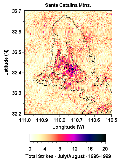
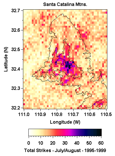
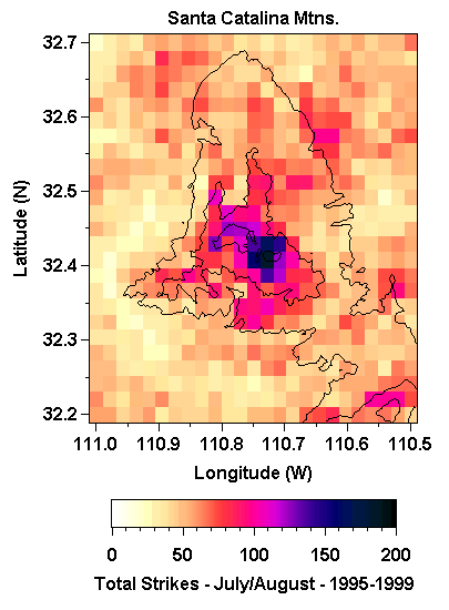 These three images represent bin sizes of 0.005 degree, 0.01
degree and 0.02 degree. The middle resolution (0.01 degree) is the
one used in the lightning maps posted at this site. The other two
plots show the results of a resolution of half as much or twice as much.
The first image shows lightning counted in bins of 0.005 degree latitude
by 0.005 degree longitude. Naturally, the smaller the grid rectangles,
the smaller the count, and the 0.005 degree grid counts will average one
fourth as much as the 0.01 degree grid. For the 0.005 grid, there
are a lot more bins where only one or two (or no) strikes occured in the
entire five year period. Even in fairly active areas, there will
be more 'holes' due to random fluctuations of the smaller numbers.
In the 0.01 degree resolution, regions of higher strike density seem to
stand out more solidly. The 0.01 degree grid rectangles give slightly
finer than 1 km resolution [about 930 m north to south and about 800 m
wide east to west]. This is just slightly beyond the typical error
in the strike locations, so one wouldn't expect to be able to go much finer
and still see any new signal in the data. The 0.02 degree plots looks
smoother yet, but the approximate 2 km x 2 km bin size is getting to be
enough bigger than the lightning location accuracy, that details of the
signals are being lost. A 4 sq. km. bin size makes for a pretty coarse
grid to lay over a small desert mountain range.
These three images represent bin sizes of 0.005 degree, 0.01
degree and 0.02 degree. The middle resolution (0.01 degree) is the
one used in the lightning maps posted at this site. The other two
plots show the results of a resolution of half as much or twice as much.
The first image shows lightning counted in bins of 0.005 degree latitude
by 0.005 degree longitude. Naturally, the smaller the grid rectangles,
the smaller the count, and the 0.005 degree grid counts will average one
fourth as much as the 0.01 degree grid. For the 0.005 grid, there
are a lot more bins where only one or two (or no) strikes occured in the
entire five year period. Even in fairly active areas, there will
be more 'holes' due to random fluctuations of the smaller numbers.
In the 0.01 degree resolution, regions of higher strike density seem to
stand out more solidly. The 0.01 degree grid rectangles give slightly
finer than 1 km resolution [about 930 m north to south and about 800 m
wide east to west]. This is just slightly beyond the typical error
in the strike locations, so one wouldn't expect to be able to go much finer
and still see any new signal in the data. The 0.02 degree plots looks
smoother yet, but the approximate 2 km x 2 km bin size is getting to be
enough bigger than the lightning location accuracy, that details of the
signals are being lost. A 4 sq. km. bin size makes for a pretty coarse
grid to lay over a small desert mountain range.
One subtle issue involves the use of fixed latitude and
longitude grids to count lightning. This is an easy method, but it
means that the area of the grid rectangle will not stay exactly fixed as
one moves from north to south. As a result the numbers, and subsequently
the colors, on these images are not strickly proportional to strike density.
There would be a tendency for the colors to get more intense at the southern
end of a map. Fortunately this tendency is very small over a single
1 degree by 2 degree quad. For example, for a quad such as Tucson,
the area of the grid rectangles increases by cos(32)/cos(33) which amounts
to 1.1%. So a 20 strike bin at the top of the Tucson quad would need
to be the same color that the value 20.22 has at the bottom of the quad,
in order for the colors to be truely proportional to strike density.
20 and 20.22 on the color scale are indistingishable, so a correction for
this effect was not made. It is a little more of an issue on maps
that cover a much larger area, such as the whole state of Arizona, but
even then it amounts to a few percent.
Total Lightning Strikes - Discussion of some Results
This section discusses one particular type of map.
These maps show total lightning strikes added up for July and August during
the five year period of 1995-1999. The strikes are totalled in a
grid of rectangles with a resolution of 0.01 degree latitude by 0.01 degree
longitude. These grid rectangles are a simple way to divide up a
quadrangle into bins, but they do have the disadvantage of changing area
as one goes from north to south. The rectangles range from as big
as 1.11 km high and 0.95 km wide (for an area of 1.05 km2) along
the southern edge and as small as 1.11 km high and 0.81 km wide (for an
area of 0.90 km2) at the northern edge. So the area of
the grid rectangles decreases about 15% from the bottom to the top of entire
region. To display an unbiased lightning density, would require correcting
for the area change.
Full Region Plots.
Figure 1. below shows lightning over the entire
region, using data that is not corrected to show the proper density.
It is a Mercator projection, so a strip across the north end is just as
wide as a strip along the south end, while in reality there is less actual
real estate for lightning to hit. This lightning is spread out into
the same number of bins so there will be a tendency for the lightning plot
to appear weaker as one moves from north to south. This turns out
to be a very small effect, however, compared to the fact that there really
is much less lightning activity over the north.
 The next graphic (Figure 2.) shows the exact same data,
but an actual density calculation has been made. The same total number
of strikes that was used to generate Figure 1. , were then divided
by the area in square kilometers of that rectangular bin. The numbers
don't change much though, since the area per bin is close to 1.0 km2
for the whole plot. In the center, especially, the area is very close
to 1.0 km2. The area is slightly more than one along the
bottom edge (1.05 km2) so these values are reduced about 5%
and the area is slightly less than one along the top edge (0.90 km2)
so these values are increased by about 10%. However, a 10% change
will turn a 20 into a 22 or a 6 into a 6.6 and a look at the color bar
shows that the difference will be hard to notice. Figure 1.
and Figure 2. are hard to tell apart. For this reason no correction
for latitude was incorpated in the results that follow. In a plot
for a single quad the correction amounts to only about 1% from the top
to the bottom which is even more trivial. All other Total Lightning
Strike maps here will use totals in 0.01 degree by 0.01 degree resolution
bins. The numbers are close to a strikes per km2 value
and that value can always be calculated more accurately, given the latitude,
if desired.
The next graphic (Figure 2.) shows the exact same data,
but an actual density calculation has been made. The same total number
of strikes that was used to generate Figure 1. , were then divided
by the area in square kilometers of that rectangular bin. The numbers
don't change much though, since the area per bin is close to 1.0 km2
for the whole plot. In the center, especially, the area is very close
to 1.0 km2. The area is slightly more than one along the
bottom edge (1.05 km2) so these values are reduced about 5%
and the area is slightly less than one along the top edge (0.90 km2)
so these values are increased by about 10%. However, a 10% change
will turn a 20 into a 22 or a 6 into a 6.6 and a look at the color bar
shows that the difference will be hard to notice. Figure 1.
and Figure 2. are hard to tell apart. For this reason no correction
for latitude was incorpated in the results that follow. In a plot
for a single quad the correction amounts to only about 1% from the top
to the bottom which is even more trivial. All other Total Lightning
Strike maps here will use totals in 0.01 degree by 0.01 degree resolution
bins. The numbers are close to a strikes per km2 value
and that value can always be calculated more accurately, given the latitude,
if desired.
 The above figures show the total lightning strikes
for the full region of study. Maps are also available at three levels
of finer detail (state regions, half state regions and quadrangle).
The detailed maps show many features that are lost on the large plot and
several examples will be seen below. The more detailed maps are especially
useful for the weaker areas, such as Utah, because the color scale can
be darkened there to enhance the weaker features. The plot of the
full region needs a color scale that spans the full range of activity.
This is also a strength of the full plot though, because it shows how the
different quads compare with each other. The separate quad plots
have color scales that use 0-20, 0-30, 0-40 or 0-50. This should
be carefully noted when viewing multiple quads.
The above figures show the total lightning strikes
for the full region of study. Maps are also available at three levels
of finer detail (state regions, half state regions and quadrangle).
The detailed maps show many features that are lost on the large plot and
several examples will be seen below. The more detailed maps are especially
useful for the weaker areas, such as Utah, because the color scale can
be darkened there to enhance the weaker features. The plot of the
full region needs a color scale that spans the full range of activity.
This is also a strength of the full plot though, because it shows how the
different quads compare with each other. The separate quad plots
have color scales that use 0-20, 0-30, 0-40 or 0-50. This should
be carefully noted when viewing multiple quads.
A number of interesting features can be seen in the plot
of the full region. There is a definite trend toward less and less
lightning as one goes from south to north. Even using the density
values to correct for shrinkage of the bin size. The highest value
in the whole plot is a 58, which is found along the lower left (in Sonora,
Mexico just south of the Nogales, AZ area). Along the northern edge
values of about 15-20 are the highest. There are several mountain
peaks that hit values of about 50 in southern Arizona and New Mexico.
These also correspond to about 50 strikes per km2. This
means about 10 strikes per km2 on an annual basis. It
should be noted that this is very high and it only includes the months
of July and August. On nationwide lightning maps, one typically only
sees values as high as 10 strikes per year per km2 in parts
of the southeast. The southeast also tends to have lightning spread
out more through the course of the year, so values of 5 strikes per month
per km2 in parts of this study region (such as the Santa Catalina
Mtns north of Tucson, AZ or the Sacremento Mtns of New Mexico) may rank
as the highest in the nation.
Figure 3. shows a plot of total lightning versus
latitude. The whole region consists of 1200 by 1200 rectangular bins
and for this plot all the bins in the same latitude row were just totalled
together. The bottom strip, for instance, has a total area of about
(1200)x(1.05 km2) = 1260 km2. The total number
of strikes in that strip was about 12,500. So this strip averaged
about 10 strikes per km2 for the five year period or about 2
strikes per year per km2. The activity drops to about
half this value at the middle of the region (the AZ/UT and NM/CO borders)
and to about a third of that value at the north edge of the region.
These values here are corrected for the decrease in bin size with latitude.
The numbers are basically a strike density with the bottom width used as
a reference so they are all strikes per 1260 km2.
 The plot of the full region also does a nice job of revealing
the lightning hot spots. There are perhaps five or so important areas
of thunderstorm development on this largest scale. Figure 4.
highlights and labels these regions. The general movement of storms
within these areas can be seen on the diurnal animations (seen and discussed
elsewhere on this site) and the arrows here are included to reflect the
overall movement trends. The five zones are discussed breifly below:
1.) The most intense activity seems to originate in the mountainous
areas along and south of the Ariz./Sonora border from Nogales to Douglas.
This activity tends to build to the NW. This area extends farther
into Mexico and the even larger mountains of the Sierra Madre, that are
too far south to be seen on these maps, probably play a role as a genesis
region.
The plot of the full region also does a nice job of revealing
the lightning hot spots. There are perhaps five or so important areas
of thunderstorm development on this largest scale. Figure 4.
highlights and labels these regions. The general movement of storms
within these areas can be seen on the diurnal animations (seen and discussed
elsewhere on this site) and the arrows here are included to reflect the
overall movement trends. The five zones are discussed breifly below:
1.) The most intense activity seems to originate in the mountainous
areas along and south of the Ariz./Sonora border from Nogales to Douglas.
This activity tends to build to the NW. This area extends farther
into Mexico and the even larger mountains of the Sierra Madre, that are
too far south to be seen on these maps, probably play a role as a genesis
region.
2.) Another large genesis area extends along the Mogollon Rim
of Arizona, through the Arizona White Mountains and ends at the Mogollon
mountains in New Mexico. Storms tend to fire first along the high
elevation axis that runs WNW to ESE and then they migrate downhill to the
SW.
3.) There is a strong genesis region in the front range mountians
around Pikes Peak which blossoms out onto the Palmer's Divide which is
a wedge of higher elevation that sticks out into the high plains.
4.) The front range mountains of northern New Mexico are also
a strong genesis region. Again the presence of a peninsula of higher
terrain heading east into the plains (the Raton Divide in this case) seems
to yield an enhanced corridor for storm development.
5.) The Sacremento Mountains of New Mexico. The diurnal
animations reveal this area as a very early genesis region. Unlike
the above mountain areas, however, storms do not seem to develop off of
these mountians in one particular direction with the strong signal seen
in those cases. In particular the extension out into the plains to
the east is not pronouced as in the other two front range areas of 3.)
and 4.).
Detailed Plots from Selected
Quads.
This section deals with the data as viewed on a much more
detailed scale. All of the maps cover only a single quad or a portion
of a quad. A number of interesting features can be seen.
Example 1.)
The first examples show a strong correlation with elevation and lightning
intensity. Figure 5. is a close-up of the Santa Catalina Mtns
just north of Tucson, AZ. These mountains are a nice example of a
large, but isolated island of high mountians (just over 9000 ft) surrounded
on all sides by lower desert (2000ft - 3000ft). The map covers an
area roughly 30 miles on each side. The lower elevations have typically
5-15 strikes per bin for the five year period, whereas the number is 3
to 5 times that at the highest zones. The lower left part of the
map would be in the city of Tucson. Note how the lightning strikes
follow the two parallel ridges that run north from the center of the mountains,
while the canyon between them is much suppressed. Sabino Canyon,
which cuts into the south side of the mountains, can also be picked out
from the lightning signal as well. The lightning maxima associated
with the Santa Catalinas appears to be centered quite well (on the average)
on the peaks with no clear trend for storms to effect the NW side or NE
side and so on.
Example 2.)
The next example (Figure 6.) shows the Sierra Estrella mountains
southwest of central Phoenix, AZ. Downtown Phoenix is in the upper
right hand portion of the map. The area covered is similar to the
previous map. Recall that each rectangular bin is close to a kilometer
square and there are 10 bins to the 0.1 degree of latitude or longitude.
The Sierra Estrellas are the mountain chain that lie along a NNW to SSE
line in the lower middle of the map. This is another isolated mountain
island surrounded by flat desert, but different in many ways from the Santa
Catalinas. The Sierra Estrellas are not nearly so high (peaking at
about 4500 ft in a 1000 ft desert plain). They are a long narrow
range, only 2 or 3 miles wide in places, while the Santa Catalinas are
much more massive, being 20-25 miles wide in any direction. Even
so the Sierra Estrellas appear to have a distinctly enhanced lightning
signal. The signal is not always very sharp each individual year
(which it is in the case of the Santa Catalinas) but has definitely emerged
after the five year period. Even the individual hot spots along the
range correspond well with the actual peaks in the mountains. There
is a lot of random scatter too, of course. Note the two hot bins
(in black) in the low desert to the west of the mountains.
There is a smaller mountain range that runs more
east to west on the middle of the right edge. This is the South Mountain
Park area and is in the Phoenix city limits. These low mountains
only reach about 2500 ft. These appear to be too small to produce
a clear lightning enhancement although there are some clusters of 'hotter'
bins around. Perhaps a weak signal would emerge in a longer time
period. The highest part of these mountains is also home to a forrest
of TV and radio towers.
Example 3.)
Clearly, a great many of the maximums and miniumums in the lightning strike
totals correspond to mountains and valleys, but there are exceptions.
Inspection of several maps will turn up a variety of blotches, streaks
or even arcs of lighting strikes that at first glance might seem to suggest
an underlying structure, but on closer examination look to be in the middle
of nowhere, topographically speaking. Random noise is to be expected,
of course, but the multi-year summation is supposed to help smooth that
out. However, five years (ten different months) is not enough to
completely smear out the contributions from individual storms. Particularly
in areas with less total lightning, that still get an occasional intense
storm (e.g. the low deserts of SW Ariz., the Colorado Plateau area of the
four corners and the high plains of New Mexico), one sees blotches and
streaks that are the signature of just one or two events. The higher
lightning activity areas do not tend to have as much fluctuation that look
like individual storms.
One of the best examples of these single storm signals
can be seen in the map below from the Ajo quadrangle (Figure 7.).
There is a pronounced peak of lightning in the NW part of the map at about
32.8 N and 113.5 W. This area is in a broad flat valley of the low
desert, near the Gila River and yet the intensity is comparible to some
of the active mountain areas in the SE part of the map. It turns
out though, that this peak is primarily due to a single tremendous storm
on Aug 27, 1997. The two plots in the image differ only in that one
does and the other does not include Aug. 27, 1997 in the five year lightning
strike totals. The large bullseye signal dissappears when that one
day is left out. It is hard to see much difference anywhere else
on the two maps, besides that storm. The Aug. 27, 1997 storm was
an unusual event. For a solid hour (5:30 MST-6:30 MST) a very intense
storm sat over the same area with 5 to 10 flashes per minute for that entire
time. Less frequent lightning occured a half hour to an hour on either
side of this period. Nothing else approaching that intensity was
seen elsewhere in the quad that day.
 In an effort to uncover these one day anomalies another
set of plots was generated. Subtracting out hand selected individual
days is not practical for all the quads, however the same information can
be obtained by counting just the number of different days with lightning
instead of the total number of strikes. That way a single storm that
produces multiple strikes in a bin will still only count for one event.
These plots are labeled 'Total Storm Days' instead of 'Total Lightning
Strikes'. The Total Storm Days plot for the Ajo area is shown below
in Figure 8. The suppression of the strong single storm maxima
is just as effective here as it was in the special plot above.
In an effort to uncover these one day anomalies another
set of plots was generated. Subtracting out hand selected individual
days is not practical for all the quads, however the same information can
be obtained by counting just the number of different days with lightning
instead of the total number of strikes. That way a single storm that
produces multiple strikes in a bin will still only count for one event.
These plots are labeled 'Total Storm Days' instead of 'Total Lightning
Strikes'. The Total Storm Days plot for the Ajo area is shown below
in Figure 8. The suppression of the strong single storm maxima
is just as effective here as it was in the special plot above.
 The Total Storm Days plot overall tends to be a little more smoothed
out, which one would expect. Still there are adjacent bins where
the number of days with lightning jump from say 2 to 12. This random
scatter is partly due to the fairly small size of the bins. It is
possible for a storm to roll through your location with heavy rain and
lightning, but if there didn't happen to be a detected cloud to ground
strike in that 1 km2 bin, it would not be counted as a storm
day.
The Total Storm Days plot overall tends to be a little more smoothed
out, which one would expect. Still there are adjacent bins where
the number of days with lightning jump from say 2 to 12. This random
scatter is partly due to the fairly small size of the bins. It is
possible for a storm to roll through your location with heavy rain and
lightning, but if there didn't happen to be a detected cloud to ground
strike in that 1 km2 bin, it would not be counted as a storm
day.
Example 4.)
Figures 9. and 10. show the Lukeville quad. The first
plot is a topographic map and the second shows lightning strikes.
This region is interesting because of the steep lightning gradient between
the Gulf of California and the mountains to the east. The Nogales
quad (to the east of Lukeville) has the highest strike densities of anywhere
in the study area, while lightning is very rare over the northern gulf.
It can be seen along the southern edge of the Lukeville lightning plot
that within a span of about forty miles (say from 112.7 W to 112.1 W) there
is five times as much lightning without a major change in the terrain.
As one travels from west to east along the south edge of the quad there
is of course a general rise in elevation and an increase in mountains but
nothing dramatic and it would seem clear that the lightning pattern reflects
something beyond just local terrain. There are mountains on both
sides of the lightning boundary and there is a large isolated volanic peak
on the quiet western side of the map. Even though this peak rivals
the highest elevations to the east, it shows only the most minimal of a
lightning signatures. This lightning gradient becomes more diffuse
to the north in Arizona. It would be interesting to see how this
feature continues farther into Mexico.
 Example 5.)
The clearest signals in the data are mountain and valley signals, but there
are other possible features to be found. Figure 11. shows
a more expanded view of the Phoenix quad. This includes the Sierra
Estrellas that were discussed above. Central Phoenix is in the NE
quarter of the plot. There are two mountain ranges to the southwest
and west of Phoenix; the Sierra Estrellas with a fairly strong maxima and
the White Tank mountains with a minimal enhancement. The Salt River
flows between these two ranges in a broad flat valley. There appears
to be an area of enhanced lightning (highlighted below) in this valley.
Storm activity in the Phoenix valley often builds down from the north,
northeast or east. As discussed earlier, the Mogollon Rim is an important
genesis area and these storms often build southwest towards the desert.
Phoenix is often at the tail end of this migration. Storms in the
valley are often preceeded by or associated with cooling outflows from
the northeast quadrant. The space between the White Tanks and Sierra
Estrellas would represent a constriction for any shallow outflows that
are generally out of the northeast. Perhaps the highlighted valley
signal is due to this convergence. The plot of Total Storm Days is
not shown here, but it looks very similar, so the enhancement is not due
to one or two anomalous storms.
Example 5.)
The clearest signals in the data are mountain and valley signals, but there
are other possible features to be found. Figure 11. shows
a more expanded view of the Phoenix quad. This includes the Sierra
Estrellas that were discussed above. Central Phoenix is in the NE
quarter of the plot. There are two mountain ranges to the southwest
and west of Phoenix; the Sierra Estrellas with a fairly strong maxima and
the White Tank mountains with a minimal enhancement. The Salt River
flows between these two ranges in a broad flat valley. There appears
to be an area of enhanced lightning (highlighted below) in this valley.
Storm activity in the Phoenix valley often builds down from the north,
northeast or east. As discussed earlier, the Mogollon Rim is an important
genesis area and these storms often build southwest towards the desert.
Phoenix is often at the tail end of this migration. Storms in the
valley are often preceeded by or associated with cooling outflows from
the northeast quadrant. The space between the White Tanks and Sierra
Estrellas would represent a constriction for any shallow outflows that
are generally out of the northeast. Perhaps the highlighted valley
signal is due to this convergence. The plot of Total Storm Days is
not shown here, but it looks very similar, so the enhancement is not due
to one or two anomalous storms.
 Example 6.)
Figures 12. and 13. show a topogrpahic map and a lightning
map for the main portion of Grand Canyon National Park, Arizona.
The south rim of the canyon represents a sharp drop-off for lightning frequency.
The north slopes inside of the canyon presents a larger complex of side
canyons and spires and the lightning reflects this. Lightning maxima
can seen with some of the pinacles inside the canyon itself, on the north
side of the river. A tendency can be seen for more lightning in the
low elevations off to the west rather than the low deserts off to the east.
This trend shows up nicely in the larger full quad maps and the diurnal
animations. The high country above the north rim turns out to be
a very early genesis area for storms, but activity here has already peaked
by 1:00 PM to 2:00 PM MST, and storms tend to develop further west and
south later. Overall, the north rim has a suprisingly weak total
signal, with more lightning found in the lower, but very rugged, mountainous
areas to the west such as the Mt. Trumbull area.
Example 6.)
Figures 12. and 13. show a topogrpahic map and a lightning
map for the main portion of Grand Canyon National Park, Arizona.
The south rim of the canyon represents a sharp drop-off for lightning frequency.
The north slopes inside of the canyon presents a larger complex of side
canyons and spires and the lightning reflects this. Lightning maxima
can seen with some of the pinacles inside the canyon itself, on the north
side of the river. A tendency can be seen for more lightning in the
low elevations off to the west rather than the low deserts off to the east.
This trend shows up nicely in the larger full quad maps and the diurnal
animations. The high country above the north rim turns out to be
a very early genesis area for storms, but activity here has already peaked
by 1:00 PM to 2:00 PM MST, and storms tend to develop further west and
south later. Overall, the north rim has a suprisingly weak total
signal, with more lightning found in the lower, but very rugged, mountainous
areas to the west such as the Mt. Trumbull area.
 Example 7.)
The next three examples illustrate a general trend that occurs from south
to north in the full region. In the southern most peaks, such as
the Sacremento Mtns in New Mexico and the Santa Catalinas Mtns in Arizona,
the lightning density is highest at or near the very highest peaks.
Farther north however, there appears to be more lightning on the side slopes
at some intermediate elevation, with a lower density at the highest elevation.
Figure 14. shows the Pikes Peak, Colorado area. Pikes Peak
is just left of the center of the map. The highest lightning activity
occurs in a rough ring around Pikes Peak. The ring forms a backwards
'C' as it wraps around the north, east and south sides of the highest peaks.
This lightning maxima occurs at an elevation that is distinctly lower than
the peak in the center.
Example 7.)
The next three examples illustrate a general trend that occurs from south
to north in the full region. In the southern most peaks, such as
the Sacremento Mtns in New Mexico and the Santa Catalinas Mtns in Arizona,
the lightning density is highest at or near the very highest peaks.
Farther north however, there appears to be more lightning on the side slopes
at some intermediate elevation, with a lower density at the highest elevation.
Figure 14. shows the Pikes Peak, Colorado area. Pikes Peak
is just left of the center of the map. The highest lightning activity
occurs in a rough ring around Pikes Peak. The ring forms a backwards
'C' as it wraps around the north, east and south sides of the highest peaks.
This lightning maxima occurs at an elevation that is distinctly lower than
the peak in the center.
 Example 8.)
Figure 15. and 16. show the Unitas Mtns in Utah. These
mountains consist of a broad, wide area of high elevation cut into with
numerous long canyons, especially on the south side. The lightning
plot shows the most frequent strikes not at the highest altitudes, but
in a rough ring around the sides. The long peninsular ridges to the
south seem to have the strongest signal. Within this middle altitude
band there are lightning minima tracing out some of the bigger canyons
on the south side.
Example 8.)
Figure 15. and 16. show the Unitas Mtns in Utah. These
mountains consist of a broad, wide area of high elevation cut into with
numerous long canyons, especially on the south side. The lightning
plot shows the most frequent strikes not at the highest altitudes, but
in a rough ring around the sides. The long peninsular ridges to the
south seem to have the strongest signal. Within this middle altitude
band there are lightning minima tracing out some of the bigger canyons
on the south side.
 Example 9.)
Figure 17. and 18. are from the far northern part of the
study region. They include the southern end of the Wind River Mountain
Range in Wyoming. This is a large prominent range but it doesn't
produce much of a signal in the lightning pattern. There is perhaps
a suggestion of lightning forming a band around the mountains at the middle
elevations as was seen in the prior examples. The western slopes
in particular seem to be enhanced. It may take more years of data
for a signal to develop at this lower lightning activity latitude.
Example 9.)
Figure 17. and 18. are from the far northern part of the
study region. They include the southern end of the Wind River Mountain
Range in Wyoming. This is a large prominent range but it doesn't
produce much of a signal in the lightning pattern. There is perhaps
a suggestion of lightning forming a band around the mountains at the middle
elevations as was seen in the prior examples. The western slopes
in particular seem to be enhanced. It may take more years of data
for a signal to develop at this lower lightning activity latitude.
 Example 10.)
These last graphics show the Mesa quad., but instead of just the five year
total, plots are also shown for each year separately. This gives
a nice picture of the year to year variation. One can also see how
the signal builds from year to year. Each year there are signs of
strong individual storms in a variety of places, but the places that end
up having a strong signal will have some contibution from each year.
The Pinal Mtns are located just below and to the right of center (about
110.7 W & 32.3 N). There is a very strong peak in 1996, but there
is some degree of enhancement all of the other years as well, thus adding
up to a definite signal.
Example 10.)
These last graphics show the Mesa quad., but instead of just the five year
total, plots are also shown for each year separately. This gives
a nice picture of the year to year variation. One can also see how
the signal builds from year to year. Each year there are signs of
strong individual storms in a variety of places, but the places that end
up having a strong signal will have some contibution from each year.
The Pinal Mtns are located just below and to the right of center (about
110.7 W & 32.3 N). There is a very strong peak in 1996, but there
is some degree of enhancement all of the other years as well, thus adding
up to a definite signal.