WATER VAPOR
WINDS IN VICINITY OF CONVECTION AND WINTER STORMS
Robert M.
Rabin1,2, Jason Brunner2, Carl Hane1,
John Haynes3
NOAA/National
Severe Storms Laboratory (NSSL), Norman, OK 1
Cooperative
Institute of Meteorological Satellite Studies (CIMSS), Madison, WI
2
Cooperative
Institute of Mesoscale Meteorological Studies (CIMMS), Norman, OK
3
ABSTRACT
Winds obtained from tracking features in satellite imagery have been used primarily to improve analyses and forecasts over ocean areas. In order to explore the use of target-tracked winds in nowcasting convection over land, the CIMSS water vapor wind tracking algorithm has been applied to GOES-8 data on an experimental basis at 30-minute intervals in near real-time over much of the U.S. The amount of editing of wind vectors has been greatly reduced in order to include larger deviations from the model 'guess' fields. This allows the detection of perturbed flow aloft due to convection and other mesoscale features not correctly captured by models.
Analyses from the wind fields include the display of wind vectors and objectively analyzed divergence, absolute and relative vorticity, and isotachs at 300 hPa. The objective analysis is based on available wind vectors and a background field from a global forecast model. Comparisons are also available between the analysed fields of divergence, vorticity, and isotachs and those from global and mesoscale forecast models. The output of these products is available on the Web and includes interactive displays.
The upper air wind
fields are examined for a variety of convective and winter storm events.
In the case of convection, the role of inertial instability is explored
by checking for zero or negative absolute vorticity and enhanced upper
level divergence during storm growth.
1. INTRODUCTION
Forecast applications of water vapor imagery have relied on the subjective interpretation of upper-level features from the imagery (Weldon, R.B., and S.J. Holmes, 1991) and comparison with their location and intensity in forecast models. Winds obtained from tracking features in the imagery have been used to improve analyses and forecasts over ocean areas. In order to explore the use of target-tracked winds in nowcasting over land, the water vapor wind tracking algorithm developed at CIMSS (Velden et al., 1997) has been applied to GOES-8 data on an experimental basis at 30-minute intervals in near real-time over much of the U.S. This is about 6 times more frequent than the operational water vapor wind products, which are produced at 3-hourly intervals. More importantly, the amount of wind vector editing has been greatly reduced in order to include larger deviations from the model 'guess' fields. This allows the detection of perturbed flow aloft due to convection and other mesoscale features not correctly captured by models.
This paper examines
the upper level wind fields deduced from water vapor imagery for a variety
of winter storms and summertime convective events. The analysis technique
is briefly described in Section 2. Results are presented in Section 3.
The study is summarized in Section 4.
2. METHOD
The first wind tracking techniques required manual interaction with the computer to identify common cloud features in successive satellite images. Wind vectors were then estimated from the displacement of features and the time interval between images. The height of each wind vector was estimated from cloud top temperature (from the window channel radiance) and vertical soundings of temperature. More recently, the process has been automated and expanded to track features in water vapor imagery. The automated technique is described in Veldon et al. (1997). It consists of target identification, height assignment, wind calculation, and editing. The automated technique relies on a background wind field to facilitate the location of common features between successive images. The Navy Operational Global Atmospheric Prediction System (NOGAPS) model (Rosmond, 1992) is used as the background field. By employing a lower resolution model such as the NOGAPS, the addition of higher resolution winds from the satellite is more clearly identifiable. For most of the cases presented in this paper, the background wind field was updated only every 6 hours. Current implementation utilizes time interpolation to provide hourly updates of the background wind field between forecast output times. It is important to note that the winds from features tracked from water vapor imagery (other than clouds) are not associated with a single altitude. Rather, these winds are representative of layers, weighted in the vertical in accordance with the weighting function of the 6.7 micron GOES image channel. Typically, most of the weight comes from a layer 200-300 hPa deep. The altitude of the weighting functions varies directly with upper level moisture. Typically, mean layer heights vary from 400 hPa in dry areas to 200 hPa where upper level moisture is high. Wind vectors directly associated with thick high clouds, such as anvil tops, are from a single level near cloud top.
Since the mean height
of wind vectors vary over a given region, it is necessary to interpolate
the values to a constant altitude before evaluation of horizontal gradients
required in the computation of kinematic parameters such as vorticity and
divergence. For this purpose, an objective analysis is used which combines
available wind vectors with the background wind field at constant pressure
levels from the NOGAPS forecast model. Grid spacing of about 100 km has
been used for the analysis. For purposes of this study, analyses centered
at 300 hPa are used for evaluation of divergence, absolute and relative
vorticity, and wind speed. This layer includes the anvil region of deep
convection where upper level divergence can be strong and related to the
mesoscale upward air motion. Because of the vertical weighting of the water
vapor winds, the derived quantities such as divergence and vorticity represent
vertical averages centered near 300 hPa. Caution should be observed in
interpreting the kinematic properties near dry areas where no satellite
winds may be available near 300 hPa. The objective analysis will be based
mainly on the background wind field in such areas. A map of wind vectors
should be examined to ensure adequate coverage.
3. ANALYSES
Analyses from the wind
fields include the display of wind vectors and objectively analyzed divergence,
absolute and relative vorticity, and isotachs at 300 hPa. The output of
these products are available in real time on the Web and includes interactive
displays (http://zonda.ssec.wisc.edu/~rabin/real.html). Comparisons are
also available between the analyzed fields of divergence, vorticity, and
isotachs and those from the NOGAPS and Rapid Update Cycle (RUC-2) model
(Benjamin et al., 1998). Color versions of the figures may be viewed
by clicking on the desired image.
3.1 Winter Storms
On 26 January 2000, a widespread area of snow developed across central Oklahoma producing 10-15 cm of accumulation (~12-23 UTC). The snowfall appeared to be related to isentropic lift associated with warm air advection. This snow event was not well predicted. It occurred well downstream of an upper level trough which moved across the region on 27 January. Snow had been forecasted (at least a couple of days in advance) to begin after 00 UTC on the 27th. The upper system produced convective precipitation further east on the 27th. Freezing rain and ice pellets effected north Texas & the heaviest snow fell in parts of eastern Oklahoma with as much as 17" reported in Eufaula, Oklahoma.
In general, the RUC-2
wind fields contain more structure than the satellite winds because of
the model's high resolution. The RUC-2's upper level divergence field seems
to match the location of the snow band on 26 January more consistently
than the satellite analysis (Fig. 1). The satellite analysis developed
a circular shaped divergent area over eastern Oklahoma by 17:45 UTC. Note
that the analyzed divergence pattern is significantly different from the
background field, which was nearly 6 hours old at the time of analysis.
The RUC-2 indicated an elongated area of divergence just south of the reflectivity
band starting by 15:45 UTC. The divergence visible from satellite may have
been limited or distorted due to the shallow nature of the upward motion
during the warm air advection phase of the storm.
|
|
|
|
Figure 1. Water vapor image and divergence at 300 hPa (10-6s-1) at 1745 UTC, 26 January 2000 from water vapor winds (top left), background wind field (top right), RUC-2 (lower left). Radar reflectivity at the same time (lower right). Maximum reflectivity is about 30 dbZ.
A strong divergence couplet develops
with the upper low as it tracks across Oklahoma by 15 UTC on 27 January
(Fig. 2). The most intense divergence is located over the convective cloud
region centered near the southeast tip of Oklahoma. Strong convergence
is located to the west near the leading edge of a dry band aloft. The RUC-2
and the background NOGAPS fields indicate the divergence further west in
western Oklahoma. Note that the background field was 3 hours old at the
time of the analysis. Despite this, the satellite analysis captured the
eastward movement and evolution of intensity.
 |
 |
 |
 |
Figure 2. Water vapor image and divergence at 300 hPa (10-6s-1) at 1545 UTC, 27 January 2000 from water vapor winds (top left), background wind field (top right), RUC-2 (lower left). Radar reflectivity at the same time (lower right). Reflectivity exceeds 40 dbZ where dark shading repeats.
Two significant snowstorms effected
the upper Midwest on 11 and 18 December 2000. The early stages of these
storms appear to have similarities from the satellite images of Figs. 3-4.
Maximum divergence developed in the central Plains ahead of the upper level
trough, convergence behind it in the Great Basin. As the storms moved east,
upper level divergence was elongated from southern Minnesota to Michigan.
In the case of 18 December at 16:45 UTC, a double maximum occurred: a western
one just ahead of the upper trough and an eastern one near a speed gradient
well north of the surface system. A surface low was located in Missouri
with a warm front extending east and south, more than 500 km south of the
divergence features. Note that both systems also exhibited an area of upper
level convergence and drying to the southwest. On the 11th, the divergence
was to the north of an east-west band of maximum vorticity. A jet maximum
was approximately 700 km to the south of the divergence maximum. Radar
echoes were widespread through the area of divergence, although only the
backside appeared to be convective from the satellite imagery. On both
days, the highest radar reflectivities were south of the area with maximum
divergence. On 18 December, the heaviest snowfall was in vicinity of the
strongest divergence (east central Wisconsin). In this case, the high reflectivities
to the south may have been due to mixed precipitation in these areas. However
on 11 December, the heaviest snowfall occurred near the Illinois-Wisconsin
border, about 100-200 km south of the maximum divergence. Here, displacement
of the divergence pattern may have been due to a slope of upward air motion
to the north with height.
 |
 |
 |
 |
Fig. 3. Satellite derived divergence
at 300 hPa (left panels) and radar reflectivity (right panels) on 11 December
2000. Top row is at 0645 UTC and bottom row at 1545 UTC.
 |
 |
 |
 |
Fig. 4. Satellite derived divergence at 300 hPa (left panels) and radar reflectivity (right panels) on 18 December 2000. Top row is at 0345 UTC and bottom row at 1245 UTC.
A severe ice storm
effected parts of Oklahoma and Arkansas on 25-26 December 2000. On the
25th at 1845 UTC, a strong upper level system was located in Arizona. Far
to the east, convective precipitation commenced from northeast Texas to
western Arkansas. Vorticity gradients were weak in this area, yet a strong
divergence signature had developed above the convection (Fig. 5). From
the isotach field, the divergence appears to result from considerable speed
gradient near the top of a ridge aloft. By the 26th at 0345 UTC, the upper
low dropped slightly to the southeast as convection and strong divergence
aloft developed to its east in New Mexico. Convection and divergence continued
to form in northeast Texas in an area of strong warm air advection under
the upper level ridge. The speed gradient appeared to be weak by this time.
A third band of convection developed between the two other bands. Initially,
upper level divergence is weak over this area. By 0945 UTC, this convection
expanded eastward and had large divergence associated with it. In this
case, the divergence resulted from considerable speed gradient ahead of
the upper level low as it moved eastward. Over the next several hours,
the upper level circulation moved east and developed a couplet of divergence,
with the divergence and heavy precipitation in Arkansas. By this time,
parts of Oklahoma and Arkansas had experienced significant upper level
lifting for as much as 36 hrs. Given subfreezing surface temperatures and
plentiful moisture, ice accumulations of several inches resulted in considerable
tree and power line damage in many locations.
 |
 |
 |
 |
 |
 |
 |
 |
 |
 |
 |
 |
Fig. 5. Satellite derived
divergence at 300 hPa (left panels) and radar reflectivity (right panels):
a) 25 December 2000 1845 UTC, b) 26 December 0345, c) 0645, d) 0945, e)
1245, f) 2345 UTC.
3.2 Warm Season Convection
An example of strong mesocale forcing occurred in Oklahoma and Kansas on 3-4 May 1999. Multiple supercell thunderstorms produced over 70 tornadoes after 2100 UTC on 3 May. Figure 6 shows upper level wind fields at 1200 UTC and early (2145 UTC) and later (0045 UTC) stages of the convective outbreak. Of interest was the wind maximum near the Oklahoma and Texas panhandles about 500 km to the west-northwest of the convection at 2145 UTC. An upper level trough was centered to the west in New Mexico and Colorado. The trough and wind maximum had moved from south central Arizona and southwest New Mexico respectively at 1200 UTC. The convection formed on the anticyclonic side of the wind maximum near a minimum in relative vorticity (-20x10-6s-1). Peaks in divergence developed over the convection and ahead of the main trough in eastern New Mexico, however the intensity was not unusually strong as compared to other convective events. By 4 May 0045 UTC, the wind maximum had shifted east and was near the western edge of the active convection. Also, the convection was centered between a couplet of cyclonic-anticyclonic vorticity. Comparisons of upper level fields were made with the operational ETA (Black, 1994) and
RUC-2 models. The models
did well in depicting the divergence above the convection and the vorticity
couplet at 00 and 06 UTC on 04 May. Earlier, there are differences between
the satellite, RUC-2 and ETA fields.
 |
 |
 |
 |
 |
 |
Fig. 6: Left panels: Wind barbs (Thick black 100-250 hPa, thin black 250-350 hPa, white 350-500 hPa) and isotachs (ms-1). Right panels: Relative vorticity (10-6s-1) in white, divergence (10-5s-1) in black, 03 May 1999: a) 1230, b) 2145 UTC, c) 04 May 1999, 00:45 UTC.
Mesoscale Convective Systems (MCS) often develop under weak upper forcing during the summer months in the U.S. Fueled by moisture and warm air advection in the low levels, they typically occur in vicinity of upper level ridges. Blanchard et al. (1998) proposed a role of inertial instability in the growth of MCSs by enhancement of upper level divergence. Using upper wind analyses from rawinsonde data, the occurrence of negative absolute vorticity, a necessary condition for inertial instability, accompanied the onset of large systems. The absolute vorticity was examined here using the satellite wind analyses for events with weak forcing.
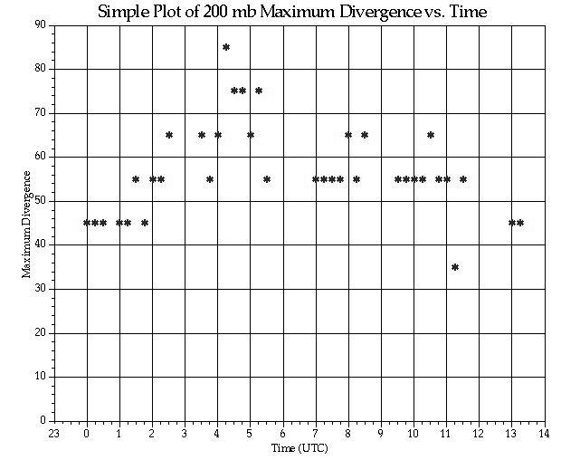
The time series of
maximum divergence was examined for a large MCS lasting 14 hours on 20
July 1995, Figure 7 (left panel). This system was associated with a frontal
boundary and had an elongated shape rather than the more circular pattern
typical of Mesoscale Convective Complexes (MCC). In this case, the time
trend of maximum divergence appears related to the evolution of the MCS
as observed from the coverage of the cold cloud shield in the infrared
satellite imagery, Figure 7 (right panel). The strongest divergence was
near the end of the mature phase (2-5 UTC). There was a rapid decline after
0530 UTC, near the onset of decay. However, the decline in divergence did
not continue during the decay phase (5-8 UTC) when values remained nearly
constant at 60x10-6. During the early stages of development
(23-03 UTC), the minimum absolute vorticity was just southeast of the convection
(Fig. 8a). Perhaps this was a factor in the observed expansion of the cloud
shield to the southeast. During the mature phase, the minimum absolute
vorticity was aligned roughly with the convection (Fig. 8b), however the
minimum was located downwind (northeast) from the most active area. In
these areas, the absolute vorticity became negative. During the decay phase,
the minimum remained aligned with the convective cloud, but was slightly
positive (Fig. 8c).
 |
 |
Fig.7. Left: Maximum
divergence (10-6s-1) vs. time. Right, top: Area of
cloud top colder than -55 C (km2), bottom: mean cloud top temperature
(K) vs. time.
Fig. 8. Divergence (black contours) and absolute vorticity (white contours), a) 2300 UTC 19 July 1995, b) 0445 UTC and c) 1315 UTC, 20 July 1995.
Another smaller, long-lived
MCS formed on 15 July 2001. The first individual convective cells formed
to the west of the upper ridge axis at 21:45 UTC. Weak divergence was first
detected at 22:15 UTC over an individual storm in the Texas panhandle (Fig.
9a). As a speed max spread northeast into Colorado, the speed shear increased
and a minimum in absolute vorticity (6-8x10⁻⁵s-1)
approached the storms from southwest . By 01:15 UTC on 16 July, the system
was comprised of a cluster of individual cells with strong divergence at
times, and absolute vorticity near 6x10⁻⁵s-1(Fig.
9b). During the period 02:45-08:15 UTC, as the cluster expanded in coverage,
the divergence was moderately high (Fig. 9c). The MCS was located near
a minimum in absolute vorticity (2-4x10⁻⁵s-1) in
southwesterly flow. This was on the anticyclonic side of a speed maximum
where the speed shear was highest. There was a vorticity maximum embedded
in the ridge further to the south, but that region was void of convective
development. The MCS moved eastward over the ridge axis during 08:45-11:15
UTC. During this period, the divergence was steady (30x10-5s-1)
(Fig. 9d). Also, the southern end moved away from minimum absolute vorticity
and weakened. The remaining portion weakened during 11:45-14:15 UTC except
for regeneration of cells near the southeast end, along the southern edge
of the speed shear. During 14:45-17:15 UTC, dissipation into cirrus occurred.
Divergence was weak during this period.
 |
 |
 |
 |
 |
 |
 |
 |
Fig. 9. Isotachs and wind barbs (left panels) and divergence and absolute vorticity (right panels) on a) 22:15 UTC 15 July 2001, b) 01:15 UTC, c) 08:15 UTC, d) 11:15 UTC 16 July 2001. Wind barbs are black (150-250 hPa), gray (250-350 hPa), and white (350-500 hPa). Divergence contours are black, absolute vorticity are white.
On 4 Jul 2000, two
individual storms evolved into an intermittent MCS (Fig. 10). These storms
were part of a long broken line east of the Rockies at 02:45 UTC. By 04:45
UTC, two clusters emerged. They merged into a single MCS by 06:45 UTC and
weakened by 08:45 UTC. There was intensification again at 10:45. The system
became diffuse by 15:45 and dissipated by 21:45. Absolute vorticity was
positive (6-8) during entire cycle. The convection was located between
local maximum and minimum in absolute vorticity. Features were weak but
can be tracked from 06:45-22:45. Divergence peaks at 07:45 near the western
edge of the consolidated storm and at 10:45 with reformation. Otherwise,
divergence was relatively weak.
 |
 |
 |
 |
 |
 |
 |
 |
Fig. 10. Same as Fig. 9 except for 04 July 2000: a) 02:45, b) 04:45, c) 06:45, d) 08:45 UTC.
The upper air features
from a long-lived MCS on 20 July 2000 tracked south of the westerlies and
appeared to be associated with new convective development after its demise
(Fig. 11). In this case, the flow is zonal without a ridge aloft. The first
system formed at 00:45 UTC and propagated along a ribbon of uniform gradient
of absolute vorticity. This was near the northern edge of the maximum speed
shear. Impressive divergence was first detected at 10:45 UTC. Convergence
developed ahead of the convection and the divergence couplet persisted
for several hours. After dissipation of the MCS (14:45 UTC), remaining
cirrus tracked southeast where new convection developed from 18:45-22:45
UTC. This convection exhibited strong divergence at times and was accompanied
by a minimum in absolute vorticity (2x10⁻⁵s-1).
 |
 |
 |
 |
 |
 |
 |
 |
 |
 |
Fig. 11. Same as Fig. 10 except for 20 July 2000: a) 00:45, b) 10:45, c) 14:45, d) 18:45, e) 22:45 UTC.
A derecho event occurred
on 9 August 2000. A small cluster of storms developed in Iowa at 5:45 UTC,
became mature by 9:45 UTC and produced wind damage (Fig.12). The system
formed and propagated east along an axis of maximum speed shear, south
of the maximum gradient of absolute vorticity (near a minimum of 4-6x10⁻⁵
s-1). New convection developed along the leading edge of the
cirrus cloud shield as it moved rapidly east toward the Atlantic coast.
Divergence was positive but weak in vicinity of the system during its lifetime.
 |
 |
 |
 |
 |
 |
Fig. 12. Same as Fig. 11 except for 09 August 2000: a) 05:45, b) 09:45, c) 13:45 UTC.
An example of an MCS which formed
near a weak vorticity maximum occurred on 19 July 2000 (Fig. 13). The first
isolated convection formed in northeast Colorado at 00:45 UTC and was accompanied
by localized divergence. The speed maximum was located just east of this
location. As the MCS reached a mature stage by 07:45 UTC, the wind speed
maximum moved further east leaving a weak speed gradient near the convection.
The convection occurred within a region of relatively high absolute vorticity
with a weak vorticity maximum nearby. The MCS decayed between 08:45-10:45
UTC in Kansas. Divergence appeared to be quite variable during the lifecycle
of this MCS.
 |
 |
 |
 |
 |
 |
Fig. 13. Same as Fig.
12 except for 19 July 2000: a) 00:45, b) 07:45, c) 10:45 UTC.
A set of shorter-lived MCSs was also examined. These all occurred near the periphery of an upper level ridge centered near the high plains.
On 3 July 2000, an
MCS formed about 03:45 UTC near the top of the ridge (Fig. 14). It rapidly
intensified an hour later and dissipated by 08:45. The absolute vorticity
became negative near the time of intensification. Moving southeastward,
the convection was on the anticyclonic side of a wind maximum (right entrance
region of the jet), located on the east side of the upper ridge. After
the demise of the convection, cirrus debris persisted at least another
13 hours. The cirrus remained centered on the location of minimum vorticity
as it propagated southeast. Scattered new convection formed underneath
this area by afternoon (21:45 UTC).
 |
 |
 |
 |
 |
 |
Fig. 14. Same as Fig. 13 except for 03 July 2000: a) 04:45, b) 08:45, c) 21:45 UTC.
Another short-lived
event formed near the top of the ridge on 11 July 2000 (Fig. 15). Convection
initiated in southern Colorado at about 20 UTC and dissipated by 03 UTC
the following day. The area of formation was collocated with a minimum
in absolute vorticity (<4x10⁻⁵) in a region of broad speed
shear. However, that feature moved east of the convection and was replaced
with increasing values (>8x10⁻⁵) by dissipation time. There
was no local wind maximum present in this case.
 |
 |
 |
 |
 |
 |
Fig. 15. Same as Fig. 14 except for 11 July 2000: a) 20:45, b) 22:45, c) 12 July 2000 0345 UTC.
An event of late morning
isolated convection occurred on 5 July 2000 (Fig. 16). Convective clusters
first formed at 11:45 UTC near northern edge of speed shear (on the anticyclonic
side of the jet). The system became mature at 15:45 UTC and weakened by
19:45 UTC. In terms of absolute vorticity, storms were located within the
ribbon of strongest gradient (4x10⁻⁵s-1/500 km) rather
than near a minimum in absolute vorticity. Regeneration of convection occurred
by 22:45 UTC further south within the absolute vorticity gradient.
 |
 |
 |
 |
 |
 |
 |
 |
Fig. 16. Same as Fig.
15 except for 5 July 2000: a) 11:45, b) 15:45, c) 19:45, d) 22:45 UTC..
4.
SUMMARY AND CONCLUSIONS
The CIMSS water vapor wind tracking algorithm has been implemented to allow the detection of perturbed flow aloft due to convection and other mesoscale features. The horizontal resolution of wind fields is limited by the density of targets which can be tracked by the automated technique, and the resolution of the objective analysis. For example, the fields of divergence and vorticity do not contain as much detail as RUC-2 analyses.
Examination of winter storm cases usually revealed a consistent relation between divergence aloft and precipitation evolution, especially near convective cloud tops. In some cases, the divergence can be displaced downwind due to shear. Areas where air ascent is limited to shallow layers may not be detectable.
Investigation of several MCS's confirm the lack of significant vorticity or divergence perturbations aloft before convective development. With areal growth of these systems, divergence and vorticity signatures emerge and occasionally persist after the demise of the active convection. Given the presence of divergence aloft on a scale of at least 200-300 km, the thunderstorm clusters usually persist for several hours over similar horizontal scales. In contrast, isolated thunderstorms are often too small to be resolved by the satellite wind analysis and appear to develop in areas with no preferred sign of divergence. However, the rapid intensification of divergence is observed occasionally with the explosive growth of a single storm.
The absolute vorticity was examined using the satellite wind analyses for events with weak forcing. In many cases, convective systems developed in the vicinity of upper ridges near minimum in absolute vorticity (with values < 4x10⁻⁵s-1). These values were only slightly above the threshold for inertial stability, suggesting a possible role of this mechanism in MCS growth. However, it is important to note that inertial instability can be ruled out in other cases where absolute vorticity was relatively high.
Derived wind fields have been made available to the NOAA Storm Prediction Center (SPC) on an experimental basis. The operational value of these products in forecasting storm evolution remains to be determined. The principal limitations of the water vapor wind analysis are the variable nature of the target heights and the lack of vertical profiling.
The future implementation
of the Geostationary Imaging Fourier Transform Spectrometer (GIFTS) by
NASA has the potential to provide analysis of water vapor winds at multiple
levels.
5. REFERENCES
Benjamin, S.G., J.M. Brown, K.J. Brundage, B.E. Schwartz, T.G. Smirnova, and T.L. Smith, 1998: The operational RUC-2. Preprints, 16th Conference on Weather Analysis and Forecasting, AMS, Phoenix, 249-252.
Black, T.L., 1994: The new NMC mesoscale Eta model: Description and forecast examples. Wea. Forecasting, 9,265-278.
Blanchard, D.O., W.R. Cotton, and J.M. Brown, 1998: Mesoscale circulation growth under conditions of weak inertial instability. Mon. Wea. Rev., 126, 118-140.
Rosmond, T.E., 1992: The design and testing of the Navy Operational Global Atmospheric Prediction System. Wea. Forecasting, 7, 262-272.
Velden, C.S., C.M. Hayden, S. Nieman, W.P. Menzel, S. Wanzong and J. Goerss, 1997: Upper-tropospheric winds derived from geostationary satellite water vapor observations. Bull. Amer. Meteor. Soc., 78, 173-195.
Weldon, R.B., and S.J.
Holmes, 1991: Water vapor imagery: Interpretation and applications to weather
analysis and forecasting. NOAA Tech. Rep. NESDIS 67, 213 pp.