 Fig. 0
How does one make probabilistic forecasts? Well, it might be just as valid to ask how does one make categorical forecasts? Let's begin with the difference between the two. In meteorological forecasting, the categorical forecast is one that has only two probabilities: zero and unity (or 0 and 100 percent). Thus, even what we call a categorical forecast can be thought of in terms of two different probabilities; such a forecast can be called dichotomous. On the other hand, the conventional interpretation of a probabilistic
forecast is one with more than two probability categories; such a forecast can be called polychotomous, to distinguish it from dichotomous forecasts. Forecasting dichotomously implies a constant certainty: 100 percent. The forecaster is implying that he or she is 100 percent certain that an event will (or will not) occur in the forecast area during the forecast period, that the afternoon high temperature will be exactly 82F, the wind will be constantly and exactly from the northeast at 8 mph, etc. Is that how you really feel when forecasting? Think about it.
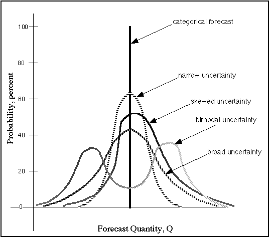
Let's assume for the sake of argument that you are forecasting some quantity, Q, at a point. This could be temperature, rainfall, etc. There are different options to take other than the standard approach of guessing what the Q-value will be. Probabilistic forecasts can take on a variety of structures. As shown in Fig. 0, it might be possible to forecast Q as a probability distribution. [Subject to the constraint that the area under the distribution always sums to unity (or 100 percent), which has not been done for the schematic figure.] The distribution can be narrow when one is relatively confident in a particular Q-value, or wide when one's certainty is relatively low. It can be skewed such that values on one side of the central peak are more likely than those on the other side, or it can even be bimodal [as with a strong quasistationary front in the vicinity when forecasting temperature]. It might be possible to make probabilistic forecasts of going past certain important threshold values of Q. Probabilistic forecasts don't all have to look like PoPs! When forecasting for an area, it is quite likely that forecast probabilities might vary from place to place, even within a single metropolitan area. That information could well be very useful to forecast customers, could it not?
If the forecast is either dichotomous or polychotomous, what about the events that we are trying to forecast? In one sense, many forecast events are dichotomous: it either rained or it did not, there was hail or there was not, a snowfall did or did not accumulate to 4 inches, it froze or it didn't, and so forth. On the other hand, the outcome of an event might be polychotomous: the observed high temperature almost any place on the planet is going to fall somewhere in a range from -100F to +120F (in increments of one degree F), measureable rainfall amounts can be anything above 0.01 inches (in increments of 0.01 inches), wind directions can be from any compass direction (usually in something like 5 degree increments from 0 to 355 degrees), an so on.
If we make up a table of forecast and observed events, such a table is called a contingency table. For the case of dichotomous forecasts and dichotomous events, it is a simple 2 x 2 table:
                                Observed (x)
 Forecast (f)   Yes (1)             No (0)           Sum
   Yes (1)      n11                  n12         n1.=n11+n12
    No (0)      n21                  n22         n2.=n21+n22
     Sum        n.1=n11+n21      n.2=n12+n22        n..=N
The occurrence of an event is given a value of unity, while the non-occurrence is given a value of zero; for these dichotomous forecasts, they also take on values of unity and zero.
If we have polychotomous forecasts (as in PoP's with, say, m categories of probability) and the event is dichotomous (it rained a measurable amount or it didn't), then the table is m x 2. If the event is also polychotomous (with, say, k categories), the table is m x k. The sums along the margins contain information about the distribution of forecasts and observations among their categories. It should be relatively easy to see how the table generalizes to polychomotous forecasts and/or events. This table contains a lot of information about how well the forecasts are doing (i.e., the verification of the forecasts). A look at verification will be deferred until later.
Think about how you do a forecast. The internal conversation you carry on with yourself as you look at weather maps is virtually always involves probabilistic concepts. It is quite natural to have uncertainty about what's going to happen.[1] And uncertainty compounds itself. You find yourself saying things like "If that front moves here by such-and-such a time, and if the moisture of a certain value comes to be near that front, then an event of a certain character is more likely than if it those conditions don't occur." This brings up the notion of conditional probability. A conditional probability is defined as the probability of one event, given that some other event has occurred. We might think of the probability of measureable rain (the standard PoP), given that the surface dewpoint reaches 55F, or whatever.
Denote probability with a "p" so that the probability of an event x is simply p(x). If we are considering a conditional probability of x, conditioned on event y, then denote that as p(x|y).
There are many different kinds of probability. The textbook example is derived from some inherent property of the system producing the event; an example is tossing a coin. Neglecting the quite unlikely outcome of the coin landing on its edge, this clearly is a dichotomous event: the coin lands either head up or tail up. Assuming an unbiased coin, the probability of either a head or a tail is obviously 50 percent. Each time we toss the coin, the probability of either outcome is always 50 percent, no matter how many times the coin is tossed. If we have had a string of 10 heads, the probability of another head is still 50 percent with the next toss. Now the frequency of any given sequence of outcomes can vary, depending on the the particular sequence, but if we are only concerned with a particular toss, the probability stays at 50 percent. This underscores the fact that there are well-defined laws for manipulating probability that allow one to work out such things as the probability of a particular sequence of coin toss outcomes. These laws of probability can be found in virtually any textbook on the subject. Outcomes can be polychotomous, of course; in the case of tossing a fair die, the probability of any particular face of the die being on top is clearly 1/6=16.6666 .... percent. And so on. This classic concept of probability arises inherently from the system being considered. It should be just as obvious that this does not apply to meteorological forecasting probabilities. We are not dealing with geometric idealizations when we look at real weather systems and processes.
Another form of probability is associated with the notion of the frequency of occurrence of events. We can return to the coin tossing example to illustrate this. If a real coin is tossed, we can collect data about such things as the frequency with which heads and tails occur, or the frequency of particular sequences of heads and tails. We believe that if we throw a fair coin enough times, the observed frequency should tend to 50 percent heads or tails, at least in the limit as the sample size becomes large. Further, we would expect a sequnce having a string of 10 heads to be much less likely than some combination of heads and tails. Is this the sort of concept we employ in weather forecasting probabilities? We don't believe so, in general. Although we certainly make use of analogs in forecasting, each weather system is basically different to a greater or lesser extent from every other weather system. Is the weather along each cold front the same as the weather along every other cold front? Not likely! Therefore, if a weather system looks similar to another one we've experienced in the past, we might think that the weather would evolve similarly, but only to a point. It would be extremely unlikely that exactly the same weather would unfold, down to the tiniest detail. In fact, this uncertainty was instrumental in the development of the ideas of "chaos" by Ed Lorenz. No matter how similar two weather systems appear to be, eventually their evolutions diverge, due to small differences in their initial states, to the point where subsequent events are as dissimilar as if they had begun with completely different initial conditions. These ideas are at the very core of notions of "predictability," a topic outside the scope of this primer.
This brings us to yet another type of probability, called subjective probability. It can be defined in a variety of ways, but the sort of definition that makes most sense in the context of weather forecasting is that the subjective probability of a particular weather event is associated with the forecaster's uncertainty that the event will occur. If one's assessment of the meteorological situation is very strongly suggestive of a particular outcome, then one's probability forecast for that event is correspondingly high. This subjective probability is just as legitimate as a probability derived from some other process, like the geometric- or frequency-derived probabilities just described. Obviously, two different forecasters might arrive at quite different subjective probabilities. Some might worry about whether their subjectively derived probabilities are right or wrong.
An important property of probability forecasts is that single forecasts using probability have no such clear sense of "right" and "wrong." That is, if it rains on a 10 percent PoP forecast, is that forecast right or wrong? Intuitively, one suspects that having it rain on a 90 percent PoP is in some sense "more right" than having it rain on a 10 percent forecast. However, this aspect of probability forecasting is only one aspect of the assessment of the performance of the forecasts. In fact, the use of probabilities precludes such a simple assessment of performance as the notion of "right vs. wrong" implies. This is a price one pays for the added flexibility and information content of using probability forecasts. Thus, the fact that on any given forecast day, two forecasters arrive at different subjective probabilities from the same data doesn't mean that one is right and the other wrong! It simply means that one is more certain of the event than the other. All this does is quantify the differences between the forecasters.
A meaningful evaluation of the performance of probability forecasts (i.e., verification) is predicated on having an ensemble of such forecasts. The property of having high PoPs out on days that rain and having low PoPs out on days that don't rain is but one aspect of a complete assessment of the forecasts. Another aspect of importance is known as reliability: reliable forecasts are those where the observed frequencies of events match the forecast probabilities. A perfectly reliable forecaster would find it rains 10 percent of the time when a 10 percent PoP forecast is issued; it would rain 20 percent of the time when a 20 percent PoP forecast is issued, etc. Such a set of forecasts means that it is quite acceptable to have it rain 10 times out of 100 forecasts of 10 percent PoPs! We'll return to this verification stuff again.
Bayes' Theorem is an important tool in using conditional probability, and is stated as follows
Bayes' Theorem: If x1, x2, ... , xm are m mutually exclusive events, of which some one must occur in a given trial, such that
 ,
,
and E is some event for which p(E) is non-zero, then
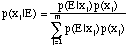 .
.
The denominator is simply p(E). Thus, this could have been written
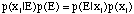 ,
,
which provides a sort of symmetry principle for conditional probabilities; the conditional probability of the event xi given event E times the unconditional probability of E is equal to the conditional probability of E given xi times the unconditional probability of xi.
If a dichotomous event is denoted by x, and the non-occurence of the event is
denoted by
 ,
then
,
then
 ,
,
and we note that p(y) + p(
 )
= 1.0. If y happens to be polychotomous such that there are m possible
values of y (and the sum of the probabilities of all of these is unity[2]), this formula can be extended to say
that
)
= 1.0. If y happens to be polychotomous such that there are m possible
values of y (and the sum of the probabilities of all of these is unity[2]), this formula can be extended to say
that
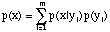 ,
,
which we have used already in Bayes' Theorem.
For the time being, let's assume that we are dealing with dichotomous events,
so we can use the simple form above. Let's consider how this works for the
event of having a tornado conditioned on the occurrence of a thunderstorm. In
both cases, the events are dichotomous; a tornado either occurs or it doesn't,
a thunderstorm either occurs or it doesn't. For all practical purposes, one
must have a thunderstorm in order to have a tornado, which means that p(x|
 )=0,
which means in turn that if we are given the separate probabilities of the
unconditional probability of a thunderstorm and the conditional probability of
a tornado given that there is a thunderstorm, we can find the unconditional
probability of a tornado by simply forming the product of those two
probabilities.
)=0,
which means in turn that if we are given the separate probabilities of the
unconditional probability of a thunderstorm and the conditional probability of
a tornado given that there is a thunderstorm, we can find the unconditional
probability of a tornado by simply forming the product of those two
probabilities.
We use this concept unconsciously all the time in arriving at our subjective probability estimates. The events we forecast are conditioned on a whole series of events occuring, none of which are absolute certainties the vast majority of the time. Hence, we must arrive at our confidence in the forecast in some way by applying Bayes' Theorem, perhaps unconsciously. Knowing Bayes' Theorem consciously might well be of value in arriving at quantative probability estimates in a careful fashion. The probability of a severe thunderstorm involves first having a thunderstorm. Given that there is a thunderstorm, we can estimate how confident we are that it would be severe. But the probability of a thunderstorm is itself conditioned by other factors[3] and those factors in turn are conditioned by still other factors. Somehow our minds are capable of integrating all these factors into a subjective estimate. Provided we do not violate any known laws of probability (e.g., using a probability outside the range from zero to unity), these mostly intuitive estimates are perfectly legitimate.
Of course, we would like to be "right" in our probability estimates, but we have seen already that this is a misleading concept in evaluating how well are estimates are performing. We really need to accumulate an ensemble of forecasts before we can say much of value about our subjective probability estimates. There are some important aspects of probability forecasting to have in mind as we go about deriving our subjective estimates of our confidence. From a certain point of view,[4] verification of our forecasts involves having information about what happened when we issued our forecasts ... in other words, we need to have filled in the contingency table. This may prove to be more challenging than it appears on the surface. There may be some uncertainty about how accurate our verification information is; for such things as severe thunderstorms and tornadoes, there are many, many reasons to believe that our current database used for verification is seriously flawed in many ways.
To the maximum extent possible, it is essential to use as verification data those observations that are directly related to the forecast. Put another way, we can only verify forecasts if we can observe the forecast events. This can be a troublesome issue, and we will deal with it further in our verification discussion. For example, PoP verification requires rainfall measurements; specfically one needs to know only whether or not at least 0.01 inches of precipitation was measured. But it is not quite so simple as that; one also must be aware of how the forecast is defined. When a PoP forecast is issued, does it only apply to the 8 inch diameter opening at the official rain guage? What does PoP really mean in the forecast? And what is the period of the forecast? It should be clear that probability of a given event goes up as the area-time product defining the forecast is increased. The probability of having a tornado somewhere in the United States during the course of an entire year is virtually indistinguishable from 100 percent. However, the probability of having a tornado in a given squre mile within Hale County, Texas between the hours of 5:00 p.m. CDT and 6:00 p.m. CDT on the 28th of May in any given year is quite small, certainly less than one percent. Therefore, one must consider the size of the area and the length of the forecast period when arriving at the estimated probability.
Moreover, we have mentioned Hale County, Texas because it has a relatively high tornado probability during late afternoons at the end of May. If we were to consider the likelihood of a tornado within a given square mile in Dupage County, Illinois between the hours of 10:00 a.m CST and 11:00 a.m CST during late January in any given year, that probability would be quite a bit lower than the Hale County example, perhaps by two orders of magnitude. In deciding on a subjective probability, having a knowledge of the climatological frequency is an important base from which to build an estimate. Is the particular meteorological situation on a given day such that the confidence in having an event is greater than or less than that of climatology? It is quite possible to imagine meteorological situations where the likelihood of a tornado within a given square mile in Dupage County, Illinois between the hours of 10:00 a.m CST and 11:00 a.m CST during late January is actually higher than that of having a tornado in a given squre mile within Hale County, Texas between the hours of 5:00 p.m. CDT and 6:00 p.m. CDT on the 28th of May. To some extent, the weather does not know anything about maps, clocks, and calendars. Thus, while knowledge of climatological frequency is an important part of establishing confidence levels in the forecast, the climatology is only a starting point and should not be taken as providing some absolute bound on the subjective estimate.
It is useful to understand that a forecast probability equal to the climatological frequency is saying that you have no information allowing you to make forecast that differs from any randomly selected situation. A climatological value is a "know-nothing" forecast! There may be times, of course, when you simply cannot distinguish anything about the situation that would allow you to choose between climatology and a higher or lower value. In such an event, it is quite acceptable to use the appropriate climatological value (which might well vary according to the location, the day of the year, and the time of day). But you should recognize what you are doing and saying about your ability to distinguish factors that would increase or lower your subjective probability relative to climatology.
Another important factor is the projection time. All other things being equal, forecasts involving longer projections have probabilities closer to climatological values as a natural consequence of limited predictability. It is tougher to forecast 48 h in advance than it is to forecast 24 h in advance. As one projects forecasts far enough into the future, it would be wise to have the subjective probabilities converge on climatology at your subjective predictability limit. What is the probability for a tornado within a given square mile in Hale County on a specific date late next May between 5:00 p.m. and 6:00 p.m. CDT? Almost certainly, the best forecast you could make would be climatology.
In this discussion, it is important to remember that the notion of time and space specificity is quite dependent on these factors. We expect to be better at probability estimation for large areas rather than small areas, for long times rather than short times, and for short projections rather than long projections, in general. Unless we have a great deal of confidence in our assessment of the meteorology, we do not want to have excessively high or low probabilities, relative to climatology. Using high probabilities over a wide area carries with it a particular implication: events will be widespread and relatively numerous within that area. If we try to be too space-specific with those high values, however, we might miss the actual location of the events; high probabilities might be warranted but if we cannot be confident in our ability to pinpoint where those high probabilities will be realized, then it is better to spread lower probabilities over a wide area.
Another important notion of probability is that it is defined over some finite area-time volume, even if the area is in some practical sense simply point measurement (recall the 8-inch rain guage!). However, it is possible to imagine a point probability forecast as an abstraction. What is the relationship between point and area probability estimates? If one establishes as a condition that __, then the area probability can be thought of as the areal coverage of the point events within that area. If one has showers over 20 percent of the forecast area, that is equivalent to an average point probability of 20 percent for all the points in the domain.
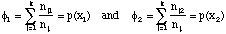
Suppose we have a meteorological event, e, for which we are forecasting. During the forecast time period, T, we have m such events, ei, i=1,2, ... ,m. If the forecast area is denoted A, then we consider the probability of one or more events in A, pA, to be the area probability; i.e., that one or more events will occur somewhere within A. As an abstraction, A is made up of an infinite number of points, with coordinates (x,y). The jth point is given by (xj,yj). If the probability of having one or more events occur at each point is finite, it is clear that pA cannot be the simple sum of the point probabilities, since that sum would be infinite (or might exceed unity)!
Consider Fig. 1. Assume that each "point" in the area is actually represented by a finite number of small sub-areas, Ak, k=1,2, ... ,n. This small subarea is the "grain size" with which we choose to resolve the total area A, which is the simple sum of the n sub-areas. The area coverage of
events during the forecast period is simply that fraction of the area which actually experiences one or more events during the forecast period, C. Mathematically, if n' is the number of subareas in which an event is observed during the period, then
 ,
,
where summation is only over those subareas affected and where the symbol "
 " denotes the intersection. At any instant, each of the ongoing events only
covers a fraction of the total area affected by events during the time T.
" denotes the intersection. At any instant, each of the ongoing events only
covers a fraction of the total area affected by events during the time T.
The forecast area coverage, Cf, is that fraction of the area we are forecasting to be affected. First of all, this does not mean we have to predict which of the subareas is going to be hit with one or more events. It simply represents our estimate of what the fractional coverage will be. Second, this is clearly a conditional forecast, being conditioned by whether at least one event actually occurs in A during T. If no event materializes, this forecast coverage has no meaning at all.
The average probability over the area A is given by
 ,
,
where the pi are the probabilities of one or more events during time T within the ith sub-area, Ai. It is assumed that the probability is uniform within a sub-area. If for some reason, the sub-areas vary in size, then each probability value must be area-weighted and the sum divided by the total area. It should be obvious that the areas associated with the sub-areas ("pseudo-points") need to be small enough that a single probability value can be applied to each. If these pseudo-point probabilities are defined on a relatively dense, regular array (e.g., the "MDR" grid), then these details tend to take care of themselves.
It is simple to show that

where it is important to note that the coverage is the forecast area
coverage. Since the expected coverage is always less than or equal to unity,
this means that the average pseudo-point probability is always less than
or equal to the area probability. But observe that from an a posteriori
point of view,
 ,
the observed area coverage. That is, average point probability within
the area A can be interpreted in terms of areal coverage. This is not of much
use to a forecaster, however, since it requires knowledge of the area coverage
before the event occurs (if an event is actually going to occur at all)!
,
the observed area coverage. That is, average point probability within
the area A can be interpreted in terms of areal coverage. This is not of much
use to a forecaster, however, since it requires knowledge of the area coverage
before the event occurs (if an event is actually going to occur at all)!
There are at least three different sorts of probability forecasts you might be called upon to make: 1) point probabilities, 2) area probabilities, and 3) probability contours. The first two are simply probability numbers. PoP forecasts, certainly the most familiar probability forecasts, are generally associated with average point probabilities (which implies a relationship to area probability and area coverage, as mentioned above). The verification of them usually involves the rainfall at a specific rain gauge, and incorporates the concepts developed above.
Although it is not generally known, the SELS outlook basically is an average point probability as well, related officially to the forecast area coverage of severe weather events. If one has "low, moderate, and high" risk categories, these are defined officially in terms of the forecast density of severe weather events within the area, or a forecast area coverage (Cf). This involves both an average point probability and the area probability, as we have shown above.
Many forecasters see probability contours associated with the TDL thunderstorm and severe thunderstorm guidance products. These have been produced using screening regression techniques on various predictor parameters and applied to events defined on the MDR grid. The predictor parameters may include such factors as climatology and observations as well as model forecast parameters.
There are other TDL guidance forecasts, including point PoPs for specific stations, contoured PoPs, and others. Whereas most forecasters are at least passingly familiar with PoPs (in spite of many misconceptions), it appears that most have little or no experience with probability contours. Thus, we want to provide at least a few tips and pointers that can help avoid some of the more egregious problems. Most of these are based on the material already presented and so are very basic. There is no way to make forecasting easy but we hope this removes some of the fear associated with unfamiliarity.
Presumably, as you begin to consider the task, you somehow formulate an intuitive sense of the likelihood of some event during your forecast period. Suppose your first thoughts on the subject look something like Fig. 2.
Figure 2. Schematic showing initial forecast probability contours.
However, you then consider that you are forecasting pretty high probabilities of the event over a pretty large area. Is it realistic to think that at least 80 percent of the pseudo-points inside your 80 percent contour are going to experience one or more events during the forecast period?[5] Perhaps not. O.K., so then you decide that you know enough to pinpoint the area pretty well. Then your forecast might look more like Fig. 3
Now you're getting really worried. The climatological frequency of this event is about 5 percent over the region you've indicated. You believe that the meteorological situation warrants a considerable increase over the climatological frequency, but are you convinced the chances are as high at 18 times the climatological frequency? Observe that 18 x 5 = 90, which would be the peak point probability you originally estimated inside your 80 percent contour. This might well seem pretty high to you. Perhaps you've decided the highest chances for an event at a point within the domain are about 7 times climatology. And you may be having second thoughts about how well you can pinpoint the area? Perhaps it would be a better forecast to cut down on the probability numbers and increase the area to reflect your geographical uncertainties. The third stage in your assessment might look more like Fig. 4.
If it turns out that you are forecasting for an event for which TDL produces a contoured probability guidance chart, you're in luck ... provided that your definition of both the forecast and the event coincide with that of TDL's chart. In that wonderful situation, the TDL chart provides you with an objective, quasi-independent assessment of the probabilities that you can use either as a point of departure or as a check on your assessment (depending on whether you look at it before or after your own look at the situation leading to your initial guess at the contours). For many forecast products, you will not be so lucky; either the event definition or the forecast definition will not be the same as that used by TDL to create their chart. However, you can still use that TDL guidance if it is in some way related to your forecast, perhaps as an assessment of the probability of some event which is similar to your forecast event, or perhaps as some related event which might be used to condition your forecast of your event.
9. Conditional probability contours
Now that you are producing probability contours, you need to consider how to use and interpret conditional probability contours. Note that some of the TDL severe thunderstorm products involve conditional probabilities. There is not necessarily some particular order in which to consider them, but suppose you have produced something like Fig. 5.
In this figure, relatively high contours of p(x|y) extend into the northwestern U.S. where the values of p(y) are relatively low. This means that the conditioning event is relatively unlikely, but if it does occur, the chances for event x are relatively high. This conveys useful information, as in situations where x=severe thunderstorm and y=thunderstorm. The meteorological factors that are associated with the conditioning event, y, may be quite different from those that affect the primary event, x, given the conditioning event. The opposite situation is also possible, where p(y) is high and p(x|y) is low. If one desires, it is possible to do the multiplications and contour the associated unconditional probabilities, p(x). This might or might not be a useful exercise, depending on the forecast.
This topic can be responsible for a lot of heartburn. We are going to consider the verification of probabilistic forecasts and not consider verification of dichotomous forecasts (the latter of which we believe to be a less than satisfactory approach for meteorologists to take).
Assuming, then, that we have decided to make probabilistic forecasts, one of the first issues we are going to have to settle upon is the probability categories. How many categories do we want to empoly and what rationale should go into deciding how to define those categories. There are several things to consider:
1. What is the climatological frequency of the event in question? Do we want roughly the same number of categories above and below the climatological frequency?
2. What are the maximum and minimum practical probability for the event? Obviously, if one knew precisely when and where things are going to occur, it would make sense to forecast only zero and unity for probabilities. This dichotomous ideal is virtually impossible to attain, which is why we are using probability in the first place, so what is practical in terms of how certain we can ever be?
3. Do we want the frequency of forecasts to be approximately constant for all categories?
4. Given that the number of categories determines our forecast "resolution," what resolution do we think we are able to attain? And what resolution is practical? Can we generate our maps of probability fast enough to meet our deadlines?
5. Do our categories convey properly our uncertainty to our users? This can be a serious problem for rare events, such a tornadoes. The climatological frequency may be so low that a realistic probability sounds like a pretty remote chance to an unsophisticated user even when the chances are many times greater than climatology. Is there a way to express the probabilities to avoid this sort of confusion?
There may well be other issues, as well. Let us assume that we somehow have arrived at a satsifactory set of probability categories, say f1, f2, ..., fk. Further, let us assume that we have managed to match our forecasts to the observations such that we have no conflict between the definition of the forecast and the definition of an event. For the sake of simplicity, we are going to consider only the occurrence and non-occurrence of our obaserved event; i.e., the observations are dichotomous. Thus, we have the k x 2 contingency table:
                                        Observed (x)
   Forecast (f)     Yes (1)             No (0)              Sum
        f1          n11                 n12                 n1.
        f2          n21                 n22                 n2.
        .           .                   .                   .
        .           .                   .                   .
        .           .                   .                   .
        fk          nk1                 nk2                 nk.
       Sum          n.1                 n.2                 n.. = N
This table contains a lot of information! In fact, Murphy argues that it contains all of the non-time-dependent information[6] we know about our verification. It is common for an assessment of the forecasts to be expressed in terms of a limited set of measures, or verification scores. This limited set of numbers typically does not begin to convey the total content of the contingency table. Therefore, Allan Murphy (and others, including us) has promoted a distributions-oriented verification that doesn't reduce the content of the table to a small set of measures. Murphy has described the complexity and dimensionality of the verification problem and it is important to note that a single measure is at best a one-dimensional consideration, whereas the real problem may be extensively multi-dimensional.
This is not the forum for a full explanation of Murphy's proposals for verification. The interested reader should consult the bibliography for pertinent details. What we want to emphasize here is that any verification that reduces the problem to one measure (or a limited set of measures) is not a particularly useful verification system. To draw on a sports analogy, suppose you own a baseball team and for whatever reason, you are considering trading away one player, and again for some reason you must choose between only two players, each of whom has been in the league for 7 years. Player R has a 0.337 lifetime batting average and scores a 100 runs per year because he is frequently on base, but averages only 5 home runs per year and 65 runs batted in. Player K has a 0.235 lifetime batting average and scores 65 runs per year, but averages 40 home runs per year and has 100 runs batted in because he hits with power when he hits. Which one is most valuable to the team? Baseball buffs (many of whom are amateur statisticians) like to create various measures of "player value" but we believe that this is a perilous exercise. Each player contributes differently to the team, and it is not easy to determine overall value (even ignoring imponderables like team spirit, etc.) using just a single measure. In the same way, looking at forecasts with a single measure easily can lead to misconceptions about how the forecasts are doing. By one measure, they may be doing well, whereas by some other measure, they're doing poorly.
As noted, our standard forecasting viewpoint is that as forecasters we often want to know what actually happened, given the forecast. This viewpoint can be expressed in terms of p(x|f), where now the values of p(x|f) are derived from the entries in the contingency table as frequencies. [Note that these probabilities are distinct from our probability categories which are the forecasts.] Thus, for example, p(x=yes (1)| f=fi) is simply ni1/n.1. The table is can then be transformed to
                                        Observed (x)
   Forecast (f)     Yes (1)             No (0)              Sum
        f1          n11/n.1             n12/n.2             f1
        f2          n21/n.1             n22/n.2             f2
        .           .                   .                   .
        .           .                   .                   .
        .           .                   .                   .
        fk          nk1/n.1             nk2/n.2             fk
       Sum          1                   1
where
 .
.
These marginal sums correspond to the frequency of forecasts in each forecast category; in the sense discussed above (in Section 2), these can be thought of as probabilities of the forecast, fi=p(fi).
However, there is another viewpoint of interest; namely, p(f|x), the probability of the forecast, given the events. This view is that of an intelligent user, who could benefit by knowing what you are likely to forecast when an event occurs versus what you are likely to forecast when the event does not occur. This can be interpreted as a "calibration" of the forecasts by the user, but it is a viewpoint of interest to the forecaster, as well. The table can be transformed in this case to
                                        Observed (x)
   Forecast (f)     Yes (1)             No (0)              Sum
        f1          n11/n1.             n12/n1.             1
        f2          n21/n2.             n22/n2.             1
        .           .                   .                   .
        .           .                   .                   .
        .           .                   .                   .
        fk          nk1/nk.             nk2/nk.             1
       Sum               [phi]1       [phi]2
where
 .
.
Note that x=x1 implies "yes" or a value of unity, and x=x2 implies "no" or a value of zero. These latter marginal sums correspond to the frequency of events and non-events, respectively; as we have just seen from the p(x|f) viewpoint, these can be thought of as probabilities of the observed events, [phi]i = p(xi).
Many things can be done with the contingency tables, especially if we are willing to look at these two different viewpoints (which correspond to what Murphy calls "factorizations"). The bibilography is the place to look for the gory details; however, forecasters who worry about their subjective probabilities can derive a lot of information from the two different factorizations of the contingency table's information. If they consider the marginal distributions of their forecasts relative to the observations, they can see if their forecasts need "calibration." It is quite likely that forecasters would make various types of mistakes in assessing subjective probabilities, and the information in these tables is the best source for an individual forecaster to assess how to improve his or her subjective probability estimates. Knowledge of the joint distribution of forecasts and events is the best mechanism to adjust one's subjective probabilities.
No matter how effective the forecasts might be, anything short of perfection leaves room for improvement. A reasonably complete verification offers forecasters the chance to go back and reconsider specific forecast failures. And successes may need reconsideration as well. Basically, the primary value of verification exercises lies in the opportunities for improvement in forecasting. Providing forecasters with feedback about their performance is important but the story definitely should not end there. If there are meteorological insights that could have been used to make better forecasts, these are most likely to be found by a careful re-examination of forecast "busts" and, perhaps to a lesser extent, forecast successes. If this important meteorological evaluation does not eventually result from the primarily statistical exercise of verification, then the statistical exercise's value is substantially reduced. Time and resources must go into verification, but then the goal should be to do the hard work of "loop-closing" by delving into meteorological reasons for success and failure on individual days.
We have said that you expect it to rain roughly 10 percent of the time you forecast a 10 percent chance of rain. And, conversely, you expect it not to rain roughly 10 percent of the time when you forecast a 90 percent chance. However, the greater the departure of the forecasts from the observations, the more concerned you should be; perfect forecasts are indeed categorical. Uncertainty is at the heart of using probabilities, but this doesn't mean that individual forecast errors are not of any concern. After all, when it rains on a 10 percent chance, that is a forecast-observation difference of 0.1-1.0 = -0.9; and when it fails to rain on a 90 percent forecast, that is a forecast-observation difference of 0.9-0.0 = +0.9. That means a substantial contribution to the RMSE, no matter how you slice it. Thus, it would not be in your best interest to, say, intentionally put out a 10 percent forecast when you thought the chances were 90 percent, simply to increase the number of rain events in your 10 percent category because the frequency of rain in your 10 percent bin was currently less than 10 percent! Hopefully, such large errors are rare, and it might well be feasible to go back and find out if there was any information in the meteorology that could have reduced the large error associated with these individual.
Naturally, this brings up the subject of "hedging." Some might interpret a probabilistic forecast as a hedge, and that is not an unreasonable position, from at least some viewpoints. However, what we are concerned with regarding "hedging" in verification is a tendency to depart from a forecaster's best judgement in a misguided effort to improve verification scores. The example just given is just such a foolish attempt; although doing so would improve the "reliability" score (perhaps), it also would increase the RMSE, and other measures, to the overall detriment of the results. In what has been referred to as a "strictly proper" verification system, a forecaster obtains his or her best verification scores when making a forecast equal to his or her best estimate. Many forecasters believe that any verificaiton system can be "played" to achieve optimal results ... if a forecaster does this, then the only real loser is the forecaster, because then the benefits to the forecaster associated with the verification exercise are lost. It is indeed possible to hedge forecasts in this way, even with a strictly proper scoring system, but when the scoring is strictly proper it is easily shown that the forecaster does more poorly overall this way than by going with the his or her best judgement.
Of course, this presumes that the forecaster has "calibrated" the forecasts by obtaining regular feedback from verification results. It is imperative that this feedback be as rapid as possible, given the constraint that a useful evaluation of probabilistic forecasts requires a reasonably large ensemble of forecasts. Hence, setting up a verification system should include a mechanism to display the results to the forecasters as soon as they are available. It would make sense that individuals could see their own tables, charts, and numbers, as well as the capability to compare their results to those of the group, but there is no obvious benefit to making every individual's data available to the group.
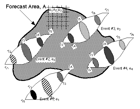 Fig. 1
 Fig. 2
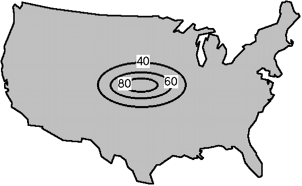 Fig. 3
 Fig. 4
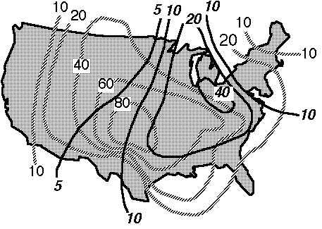 Fig. 5