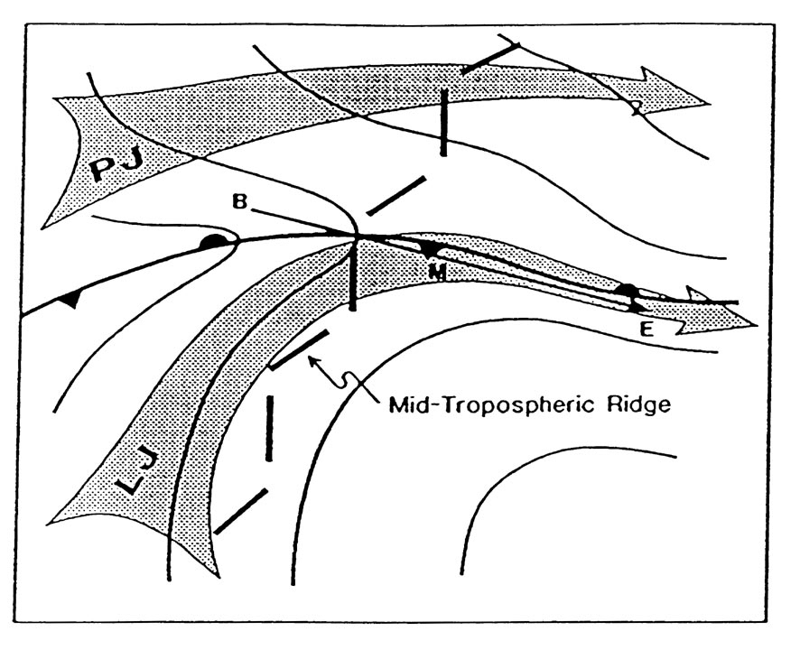
Fig. 1. Top panel: Idealized sketch of a midlatitude warm season synoptic-scale pattern favorable for the development of especially severe and long-lived progressive derechos. The line B-M-E represents the track of the derecho. Bottom panel: As in top panel, except for situations favorable for the development of squall lines with extensive bow echo-induced damaging winds (serial derechos). The thin lines denote sea level isobars in the vicinity of a quasi-stationary frontal boundary. Broad arrows represent low-level jet stream (LJ), the polar jet (PJ) and the subtropical jet (SJ). (after Johns 1993).

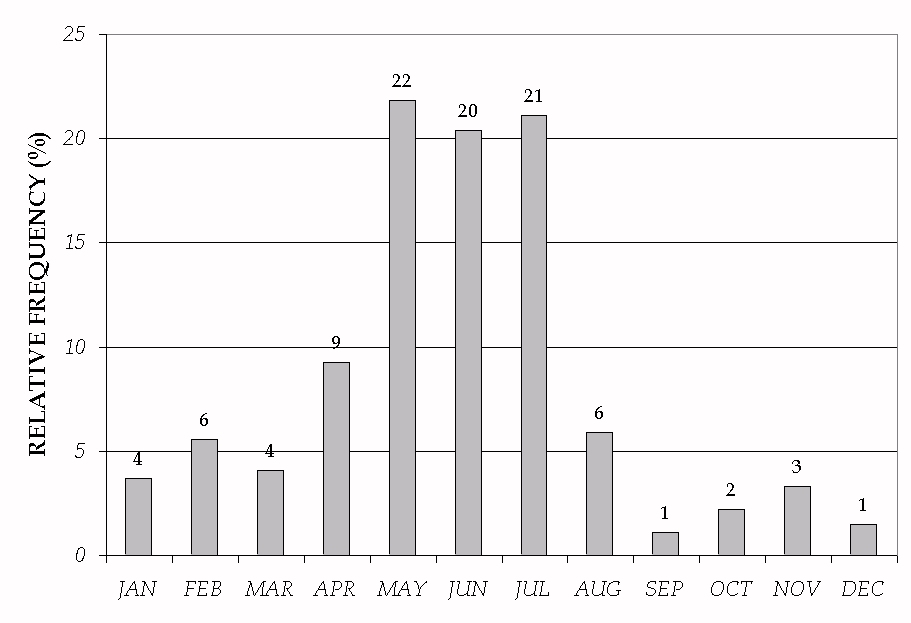
Fig. 2. The relative frequency distribution of the month of occurrence for the 270 derecho events.

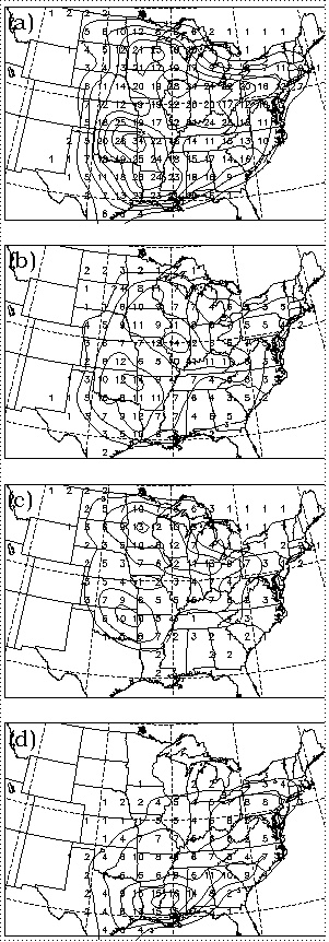
Fig. 3. The total number of derechos in 200 km by 200 km squares for, (a) all 270 events, (b) the 114 events during the months of May and June, (c) the 73 events during the months of July and August, and (d) the 83 events during the months of September through April. Contours are drawn every 4 events in (a) and every 3 events in (b), (c), and (d).

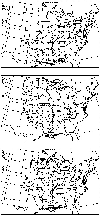
Fig. 4. The total number of derechos in 200 km by 200 km squares for (a) the 91 cases in the upstream-trough pattern, (b) the 46 cases in the ridge pattern, and (c) the 28 cases in the zonal pattern. Contours are drawn every 3 events in (a), every 2 events in (b), and every 1 event in (c).

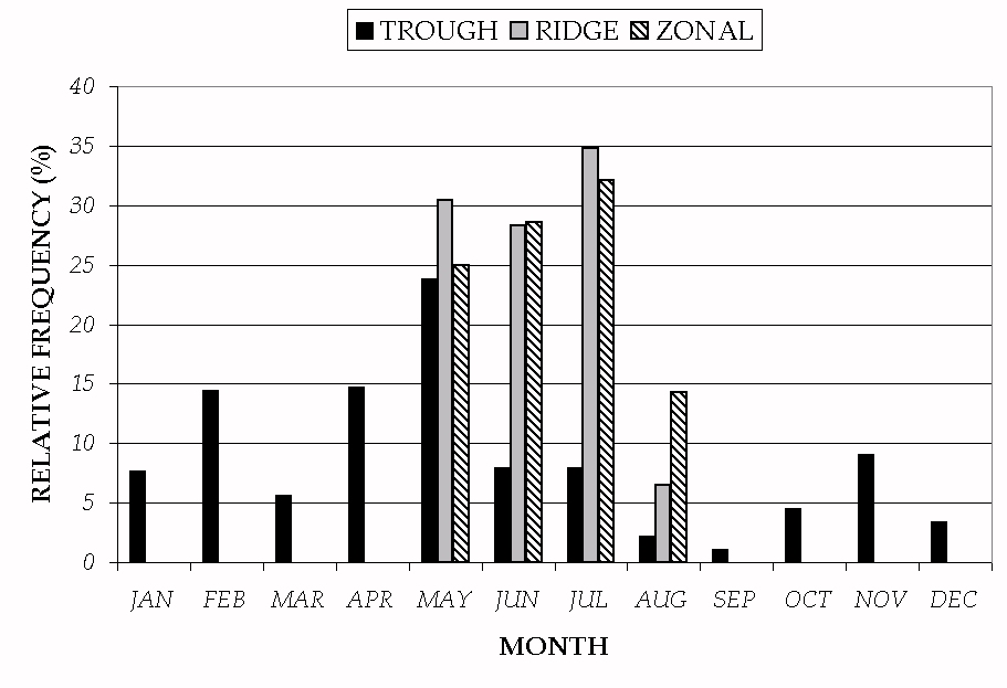
 Fig. 5. The relative frequency distributions of the derecho month of occurrence among the upstream-trough, ridge, and zonal patterns.

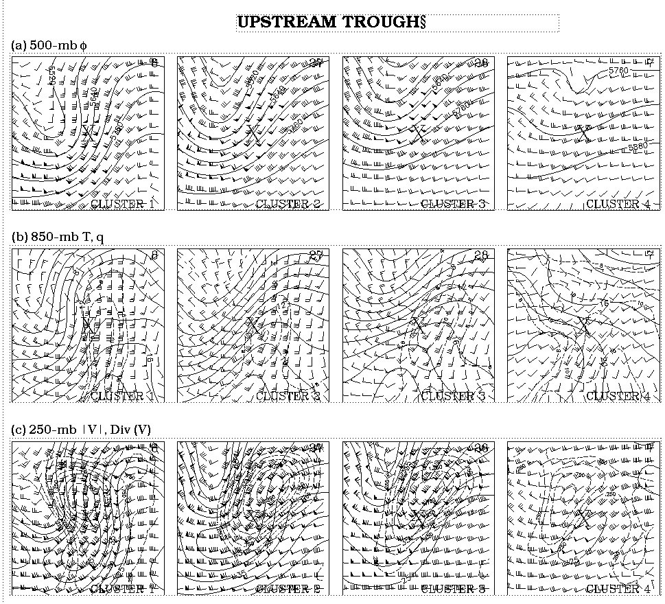
 Fig. 6. (a) The mean 500-mb geopotential height (f , contours every 60 m) and wind (flag = 25 m s^-1, full barb = 5 m s^-1) for 4 clusters within the upstream-trough pattern. (b) As in (a), except for the 850-mb temperature (T, solid contours every 2 K) and specific humidity (q, dashed contours every 1 g kg^-1 starting at 8 g kg^-1). (c) As in (a), except for the 250-mb wind speed (|V|, solid contours every 5 m s^-1, starting at 25 m s^-1) and divergence of the wind (Div (V), dashed contours every 0.25 x 10^-5 s^-1). The horizontal and vertical dimension of each grid is 2600 km by 2400 km, respectively. The X denotes the mean position of the DCS at the analysis time. The number in the upper-right corner of each grid denotes the number of analyses in each composite (cluster).

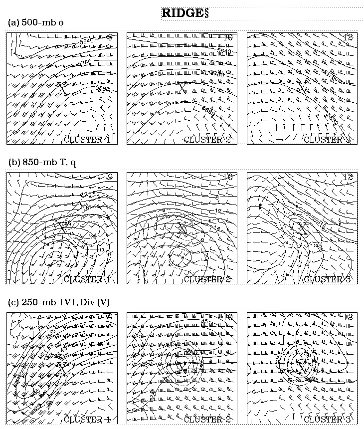
Fig. 7. As in Fig. 6, except for the ridge pattern.

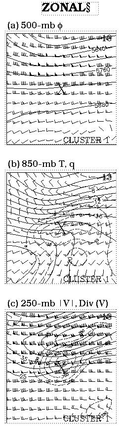
Fig. 8. As in Fig. 6, except for the zonal pattern.

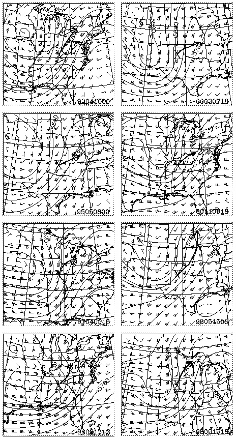
Fig. 9. The 500-mb geopotential height and wind (as in Fig. 6) for the 8 cases that comprise cluster 1 in the upstream-trough pattern. The X denotes the approximate location of the DCS at the analysis time and the arrow depicts the approximate track of the derecho major axis. The time of each analysis (UTC in YYMMDDHH format) is displayed in the lower right of each panel.

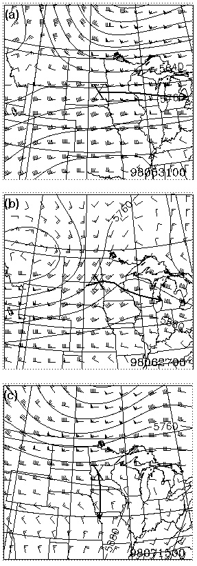
Fig. 10. Examples of 500-mb geopotential heights and winds from hybrid patterns. (a) An example of an upstream-trough/zonal pattern hybrid. (b) An example of an upstream-trough/ridge pattern hybrid. (c) An example of an unclassifiable hybrid pattern. The approximate track of the derecho major axis is depicted by the arrow. The time of each analysis (UTC in YYMMDDHH format) is displayed in the lower right of each panel.

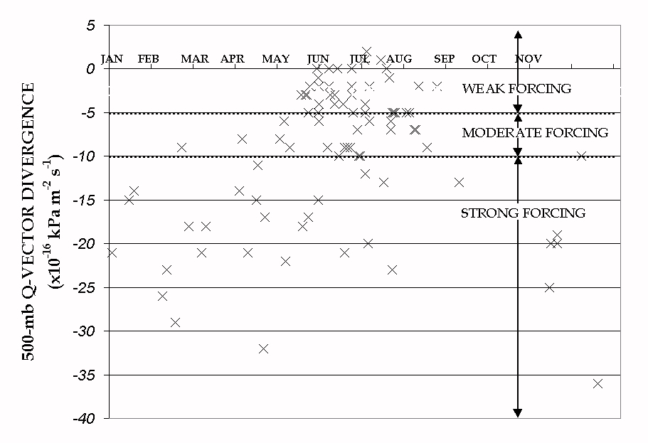
Fig. 11. The distribution of the mean 500-mb Q-vector divergence (scaled by 10¹⁶ kPa m^-2 s^-1) versus day associated with the 91 beginning and mature proximity soundings. The thresholds for defining the forcing stratification are shown by the dashed lines.

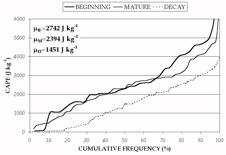
Fig. 12. The cumulative frequency distribution of CAPE (J kg^-1) for the beginning, mature, and decay soundings. The sample means for the beginning (m_B), mature (m_M), and the decay (m_D) soundings are shown in the upper left-hand corner. m_D is significantly different than both m_B and m_M at the 95% confidence level.

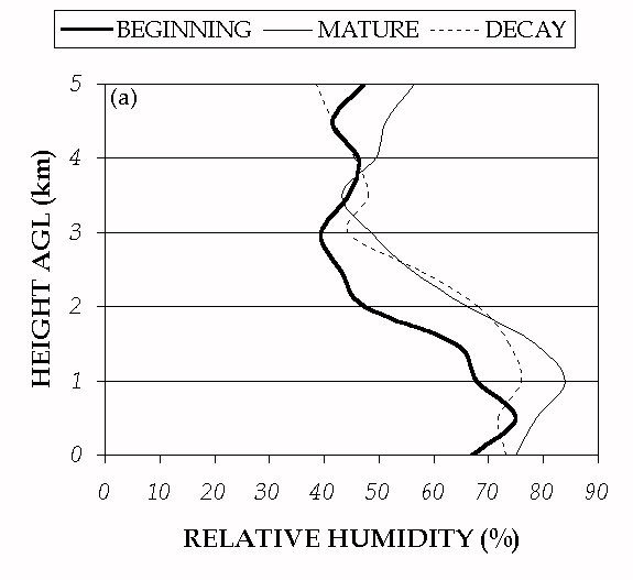
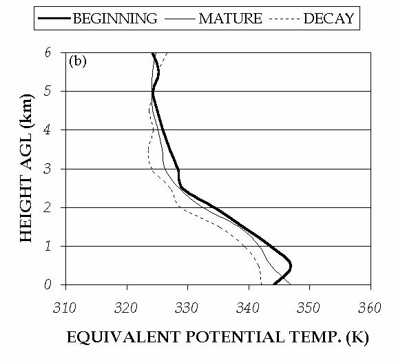
Fig. 13. Vertical profiles of (a) median RH and (b) q _e for the beginning, mature, and decay sondings. The beginning and mature RH profiles are statistically different at the 95% confidence level between 0.75 and 3 km. There are no statistically significant differences in the q _e profiles.

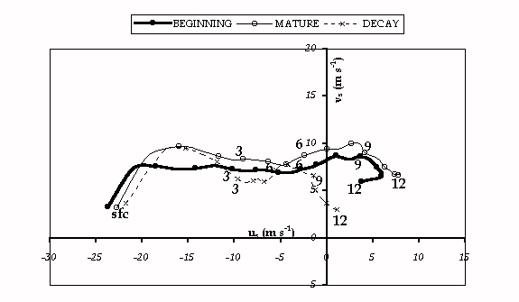
Fig. 14. Mean hodographs for the beginning, mature, and decay soundings. Prior to averaging, the wind components (u,v) in each sounding are represented in a coordinate system with the tip of the mean MCS motion vector (u_s,v_s) at the origin. The mean winds are calculated every 0.5 km above ground level (AGL), are plotted every 1 km

AGL, and are labeled every 3 km AGL. Mean shear values related to the mean hodographs are given in Table 1.

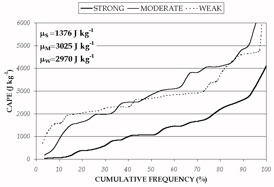
Fig. 15. The cumulative frequency distribution of CAPE (J kg^-1) for the strong, moderate, and weak-forcing soundings. The sample means for the strong (m_S), moderate (m_M), and the weak (m_W) forcing soundings are shown in the upper right corner. m_S is significantly different than both m_M and m_W at the 95% confidence level.

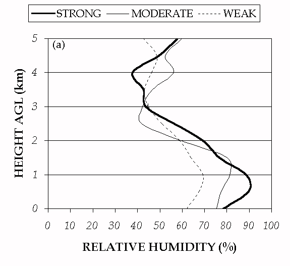
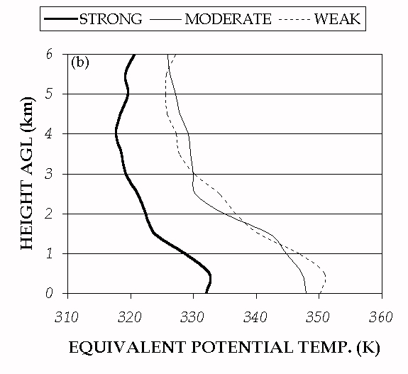
Fig. 16. As in Fig. 13, except for the strong, moderate, and weak forcing soundings. The strong and weak forcing profiles are statistically different at the 95% confidence level between the surface and 1.25 km. The strong forcing q _e profile is significantly different from the moderate and weak forcing q _e profiles at the 95% confidence level at all vertical levels (0-6 km).

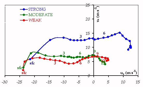
Fig. 17. As in Fig. 14, except for the strong, moderate, and weak forcing soundings. Mean shear values are given in Table 1.

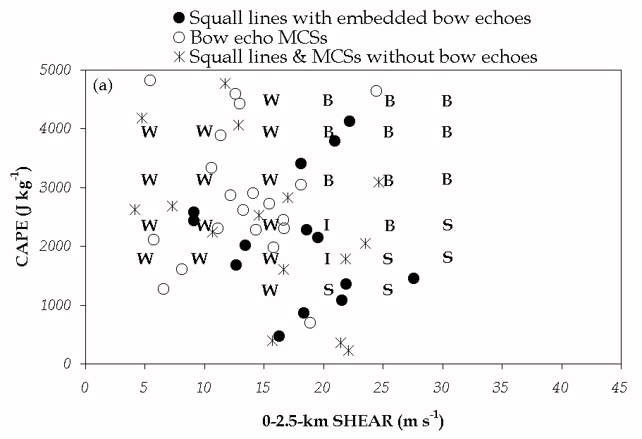
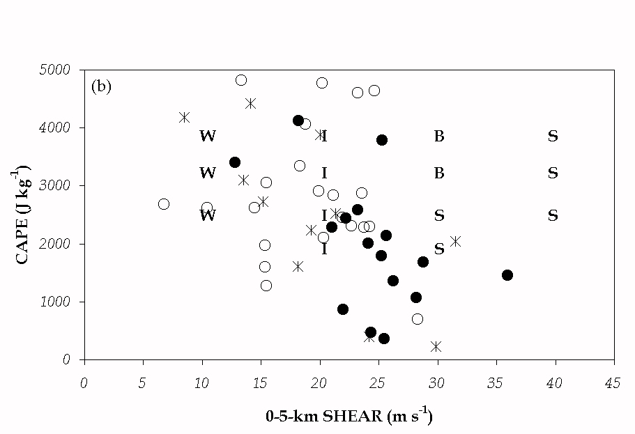
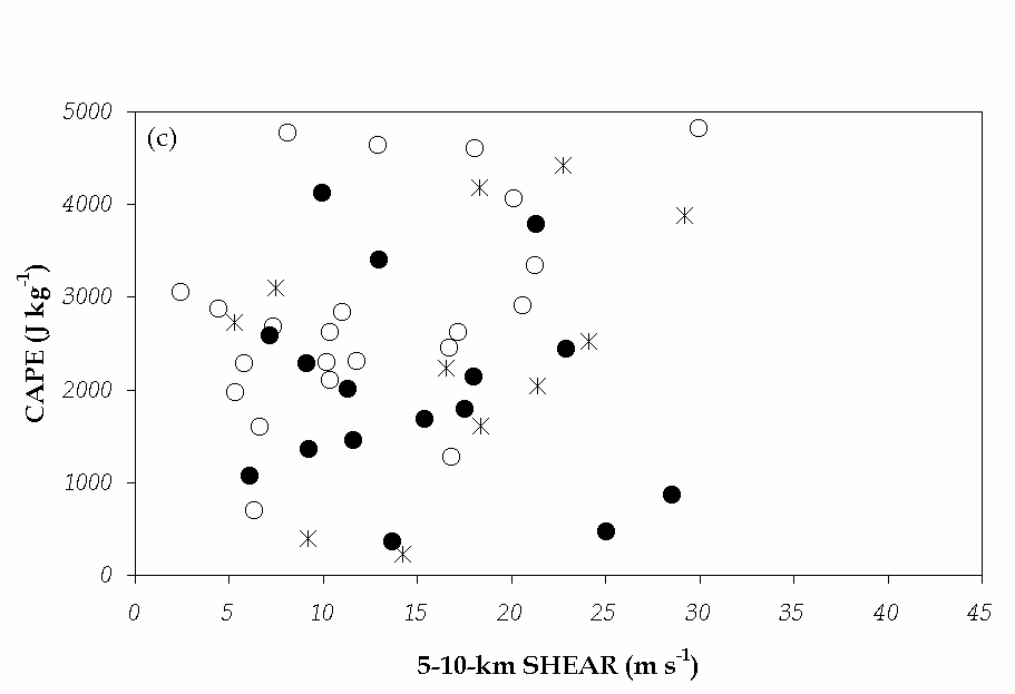
Fig. 18. Scatterplots of (a) 0-2.5 km, (b) 0-5 km, and (c) 5-10 km shear vector magnitudes (m s^-1) versus CAPE (J kg^-1) for those soundings in which the convective structure of the DCS is identified (see legend at top of figure). Results from Weisman’s (1993) numerical simulations of convective systems also are shown in (a) and (b) (see his Fig. 24). The letters represent the convective structure of the simulated systems as defined by Weisman (1993) (see text for details).